Image classification via fine-tuning with EfficientNet
Author: Yixing Fu
Date created: 2020/06/30
Last modified: 2023/07/10
Description: Use EfficientNet with weights pre-trained on imagenet for Stanford Dogs classification.

Introduction: what is EfficientNet
EfficientNet, first introduced in Tan and Le, 2019 is among the most efficient models (i.e. requiring least FLOPS for inference) that reaches State-of-the-Art accuracy on both imagenet and common image classification transfer learning tasks.
The smallest base model is similar to MnasNet, which reached near-SOTA with a significantly smaller model. By introducing a heuristic way to scale the model, EfficientNet provides a family of models (B0 to B7) that represents a good combination of efficiency and accuracy on a variety of scales. Such a scaling heuristics (compound-scaling, details see Tan and Le, 2019) allows the efficiency-oriented base model (B0) to surpass models at every scale, while avoiding extensive grid-search of hyperparameters.
A summary of the latest updates on the model is available at here, where various augmentation schemes and semi-supervised learning approaches are applied to further improve the imagenet performance of the models. These extensions of the model can be used by updating weights without changing model architecture.
B0 to B7 variants of EfficientNet
(This section provides some details on "compound scaling", and can be skipped if you're only interested in using the models)
Based on the original paper people may have the impression that EfficientNet is a continuous family of models created by arbitrarily choosing scaling factor in as Eq.(3) of the paper. However, choice of resolution, depth and width are also restricted by many factors:
- Resolution: Resolutions not divisible by 8, 16, etc. cause zero-padding near boundaries of some layers which wastes computational resources. This especially applies to smaller variants of the model, hence the input resolution for B0 and B1 are chosen as 224 and 240.
- Depth and width: The building blocks of EfficientNet demands channel size to be multiples of 8.
- Resource limit: Memory limitation may bottleneck resolution when depth and width can still increase. In such a situation, increasing depth and/or width but keep resolution can still improve performance.
As a result, the depth, width and resolution of each variant of the EfficientNet models are hand-picked and proven to produce good results, though they may be significantly off from the compound scaling formula. Therefore, the keras implementation (detailed below) only provide these 8 models, B0 to B7, instead of allowing arbitray choice of width / depth / resolution parameters.
Keras implementation of EfficientNet
An implementation of EfficientNet B0 to B7 has been shipped with Keras since v2.3. To use EfficientNetB0 for classifying 1000 classes of images from ImageNet, run:
from tensorflow.keras.applications import EfficientNetB0
model = EfficientNetB0(weights='imagenet')
This model takes input images of shape (224, 224, 3), and the input data should be in the
range [0, 255]. Normalization is included as part of the model.
Because training EfficientNet on ImageNet takes a tremendous amount of resources and several techniques that are not a part of the model architecture itself. Hence the Keras implementation by default loads pre-trained weights obtained via training with AutoAugment.
For B0 to B7 base models, the input shapes are different. Here is a list of input shape expected for each model:
| Base model | resolution |
|---|---|
| EfficientNetB0 | 224 |
| EfficientNetB1 | 240 |
| EfficientNetB2 | 260 |
| EfficientNetB3 | 300 |
| EfficientNetB4 | 380 |
| EfficientNetB5 | 456 |
| EfficientNetB6 | 528 |
| EfficientNetB7 | 600 |
When the model is intended for transfer learning, the Keras implementation provides a option to remove the top layers:
model = EfficientNetB0(include_top=False, weights='imagenet')
This option excludes the final Dense layer that turns 1280 features on the penultimate
layer into prediction of the 1000 ImageNet classes. Replacing the top layer with custom
layers allows using EfficientNet as a feature extractor in a transfer learning workflow.
Another argument in the model constructor worth noticing is drop_connect_rate which controls
the dropout rate responsible for stochastic depth.
This parameter serves as a toggle for extra regularization in finetuning, but does not
affect loaded weights. For example, when stronger regularization is desired, try:
model = EfficientNetB0(weights='imagenet', drop_connect_rate=0.4)
The default value is 0.2.
Example: EfficientNetB0 for Stanford Dogs.
EfficientNet is capable of a wide range of image classification tasks. This makes it a good model for transfer learning. As an end-to-end example, we will show using pre-trained EfficientNetB0 on Stanford Dogs dataset.
Setup and data loading
import numpy as np
import tensorflow_datasets as tfds
import tensorflow as tf  # For tf.data
import matplotlib.pyplot as plt
import keras
from keras import layers
from keras.applications import EfficientNetB0

# IMG_SIZE is determined by EfficientNet model choice
IMG_SIZE = 224
BATCH_SIZE = 64
Loading data
Here we load data from tensorflow_datasets (hereafter TFDS). Stanford Dogs dataset is provided in TFDS as stanford_dogs. It features 20,580 images that belong to 120 classes of dog breeds (12,000 for training and 8,580 for testing).
By simply changing dataset_name below, you may also try this notebook for
other datasets in TFDS such as
cifar10,
cifar100,
food101,
etc. When the images are much smaller than the size of EfficientNet input,
we can simply upsample the input images. It has been shown in
Tan and Le, 2019 that transfer learning
result is better for increased resolution even if input images remain small.
dataset_name = "stanford_dogs"
(ds_train, ds_test), ds_info = tfds.load(
    dataset_name, split=["train", "test"], with_info=True, as_supervised=True
)
NUM_CLASSES = ds_info.features["label"].num_classes
When the dataset include images with various size, we need to resize them into a shared size. The Stanford Dogs dataset includes only images at least 200x200 pixels in size. Here we resize the images to the input size needed for EfficientNet.
size = (IMG_SIZE, IMG_SIZE)
ds_train = ds_train.map(lambda image, label: (tf.image.resize(image, size), label))
ds_test = ds_test.map(lambda image, label: (tf.image.resize(image, size), label))
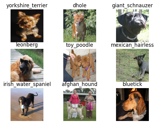
Visualizing the data
The following code shows the first 9 images with their labels.
def format_label(label):
    string_label = label_info.int2str(label)
    return string_label.split("-")[1]


label_info = ds_info.features["label"]
for i, (image, label) in enumerate(ds_train.take(9)):
    ax = plt.subplot(3, 3, i + 1)
    plt.imshow(image.numpy().astype("uint8"))
    plt.title("{}".format(format_label(label)))
    plt.axis("off")
Data augmentation
We can use the preprocessing layers APIs for image augmentation.
img_augmentation_layers = [
    layers.RandomRotation(factor=0.15),
    layers.RandomTranslation(height_factor=0.1, width_factor=0.1),
    layers.RandomFlip(),
    layers.RandomContrast(factor=0.1),
]


def img_augmentation(images):
    for layer in img_augmentation_layers:
        images = layer(images)
    return images
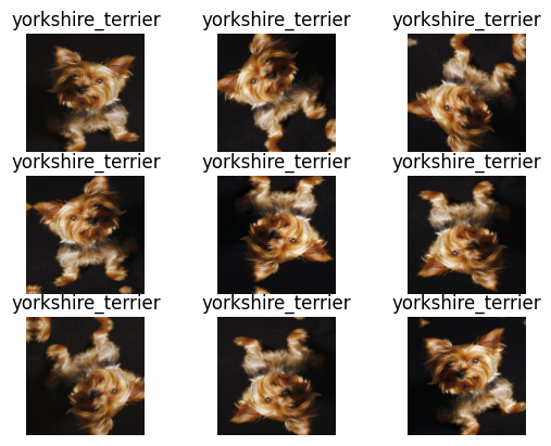
This Sequential model object can be used both as a part of
the model we later build, and as a function to preprocess
data before feeding into the model. Using them as function makes
it easy to visualize the augmented images. Here we plot 9 examples
of augmentation result of a given figure.
for image, label in ds_train.take(1):
    for i in range(9):
        ax = plt.subplot(3, 3, i + 1)
        aug_img = img_augmentation(np.expand_dims(image.numpy(), axis=0))
        aug_img = np.array(aug_img)
        plt.imshow(aug_img[0].astype("uint8"))
        plt.title("{}".format(format_label(label)))
        plt.axis("off")
Prepare inputs
Once we verify the input data and augmentation are working correctly,
we prepare dataset for training. The input data are resized to uniform
IMG_SIZE. The labels are put into one-hot
(a.k.a. categorical) encoding. The dataset is batched.
Note: prefetch and AUTOTUNE may in some situation improve
performance, but depends on environment and the specific dataset used.
See this guide
for more information on data pipeline performance.
# One-hot / categorical encoding
def input_preprocess_train(image, label):
    image = img_augmentation(image)
    label = tf.one_hot(label, NUM_CLASSES)
    return image, label


def input_preprocess_test(image, label):
    label = tf.one_hot(label, NUM_CLASSES)
    return image, label


ds_train = ds_train.map(input_preprocess_train, num_parallel_calls=tf.data.AUTOTUNE)
ds_train = ds_train.batch(batch_size=BATCH_SIZE, drop_remainder=True)
ds_train = ds_train.prefetch(tf.data.AUTOTUNE)

ds_test = ds_test.map(input_preprocess_test, num_parallel_calls=tf.data.AUTOTUNE)
ds_test = ds_test.batch(batch_size=BATCH_SIZE, drop_remainder=True)
Training a model from scratch
We build an EfficientNetB0 with 120 output classes, that is initialized from scratch:
Note: the accuracy will increase very slowly and may overfit.
model = EfficientNetB0(
    include_top=True,
    weights=None,
    classes=NUM_CLASSES,
    input_shape=(IMG_SIZE, IMG_SIZE, 3),
)
model.compile(optimizer="adam", loss="categorical_crossentropy", metrics=["accuracy"])

model.summary()

epochs = 40  # @param {type: "slider", min:10, max:100}
hist = model.fit(ds_train, epochs=epochs, validation_data=ds_test)
Model: "efficientnetb0"
┏━━━━━━━━━━━━━━━━━━━━━┳━━━━━━━━━━━━━━━━━━━┳━━━━━━━━━┳━━━━━━━━━━━━━━━━━━━━━━┓ ┃ Layer (type) ┃ Output Shape ┃ Param # ┃ Connected to ┃ ┡━━━━━━━━━━━━━━━━━━━━━╇━━━━━━━━━━━━━━━━━━━╇━━━━━━━━━╇━━━━━━━━━━━━━━━━━━━━━━┩ │ input_layer │ (None, 224, 224, │ 0 │ - │ │ (InputLayer) │ 3) │ │ │ ├─────────────────────┼───────────────────┼─────────┼──────────────────────┤ │ rescaling │ (None, 224, 224, │ 0 │ input_layer[0][0] │ │ (Rescaling) │ 3) │ │ │ ├─────────────────────┼───────────────────┼─────────┼──────────────────────┤ │ normalization │ (None, 224, 224, │ 7 │ rescaling[0][0] │ │ (Normalization) │ 3) │ │ │ ├─────────────────────┼───────────────────┼─────────┼──────────────────────┤ │ stem_conv_pad │ (None, 225, 225, │ 0 │ normalization[0][0] │ │ (ZeroPadding2D) │ 3) │ │ │ ├─────────────────────┼───────────────────┼─────────┼──────────────────────┤ │ stem_conv (Conv2D) │ (None, 112, 112, │ 864 │ stem_conv_pad[0][0] │ │ │ 32) │ │ │ ├─────────────────────┼───────────────────┼─────────┼──────────────────────┤ │ stem_bn │ (None, 112, 112, │ 128 │ stem_conv[0][0] │ │ (BatchNormalizatio… │ 32) │ │ │ ├─────────────────────┼───────────────────┼─────────┼──────────────────────┤ │ stem_activation │ (None, 112, 112, │ 0 │ stem_bn[0][0] │ │ (Activation) │ 32) │ │ │ ├─────────────────────┼───────────────────┼─────────┼──────────────────────┤ │ block1a_dwconv │ (None, 112, 112, │ 288 │ stem_activation[0][… │ │ (DepthwiseConv2D) │ 32) │ │ │ ├─────────────────────┼───────────────────┼─────────┼──────────────────────┤ │ block1a_bn │ (None, 112, 112, │ 128 │ block1a_dwconv[0][0] │ │ (BatchNormalizatio… │ 32) │ │ │ ├─────────────────────┼───────────────────┼─────────┼──────────────────────┤ │ block1a_activation │ (None, 112, 112, │ 0 │ block1a_bn[0][0] │ │ (Activation) │ 32) │ │ │ ├─────────────────────┼───────────────────┼─────────┼──────────────────────┤ │ block1a_se_squeeze │ (None, 32) │ 0 │ block1a_activation[… │ │ (GlobalAveragePool… │ │ │ │ ├─────────────────────┼───────────────────┼─────────┼──────────────────────┤ │ block1a_se_reshape │ (None, 1, 1, 32) │ 0 │ block1a_se_squeeze[… │ │ (Reshape) │ │ │ │ ├─────────────────────┼───────────────────┼─────────┼──────────────────────┤ │ block1a_se_reduce │ (None, 1, 1, 8) │ 264 │ block1a_se_reshape[… │ │ (Conv2D) │ │ │ │ ├─────────────────────┼───────────────────┼─────────┼──────────────────────┤ │ block1a_se_expand │ (None, 1, 1, 32) │ 288 │ block1a_se_reduce[0… │ │ (Conv2D) │ │ │ │ ├─────────────────────┼───────────────────┼─────────┼──────────────────────┤ │ block1a_se_excite │ (None, 112, 112, │ 0 │ block1a_activation[… │ │ (Multiply) │ 32) │ │ block1a_se_expand[0… │ ├─────────────────────┼───────────────────┼─────────┼──────────────────────┤ │ block1a_project_co… │ (None, 112, 112, │ 512 │ block1a_se_excite[0… │ │ (Conv2D) │ 16) │ │ │ ├─────────────────────┼───────────────────┼─────────┼──────────────────────┤ │ block1a_project_bn │ (None, 112, 112, │ 64 │ block1a_project_con… │ │ (BatchNormalizatio… │ 16) │ │ │ ├─────────────────────┼───────────────────┼─────────┼──────────────────────┤ │ block2a_expand_conv │ (None, 112, 112, │ 1,536 │ block1a_project_bn[… │ │ (Conv2D) │ 96) │ │ │ ├─────────────────────┼───────────────────┼─────────┼──────────────────────┤ │ block2a_expand_bn │ (None, 112, 112, │ 384 │ block2a_expand_conv… │ │ (BatchNormalizatio… │ 96) │ │ │ ├─────────────────────┼───────────────────┼─────────┼──────────────────────┤ │ block2a_expand_act… │ (None, 112, 112, │ 0 │ block2a_expand_bn[0… │ │ (Activation) │ 96) │ │ │ ├─────────────────────┼───────────────────┼─────────┼──────────────────────┤ │ block2a_dwconv_pad │ (None, 113, 113, │ 0 │ block2a_expand_acti… │ │ (ZeroPadding2D) │ 96) │ │ │ ├─────────────────────┼───────────────────┼─────────┼──────────────────────┤ │ block2a_dwconv │ (None, 56, 56, │ 864 │ block2a_dwconv_pad[… │ │ (DepthwiseConv2D) │ 96) │ │ │ ├─────────────────────┼───────────────────┼─────────┼──────────────────────┤ │ block2a_bn │ (None, 56, 56, │ 384 │ block2a_dwconv[0][0] │ │ (BatchNormalizatio… │ 96) │ │ │ ├─────────────────────┼───────────────────┼─────────┼──────────────────────┤ │ block2a_activation │ (None, 56, 56, │ 0 │ block2a_bn[0][0] │ │ (Activation) │ 96) │ │ │ ├─────────────────────┼───────────────────┼─────────┼──────────────────────┤ │ block2a_se_squeeze │ (None, 96) │ 0 │ block2a_activation[… │ │ (GlobalAveragePool… │ │ │ │ ├─────────────────────┼───────────────────┼─────────┼──────────────────────┤ │ block2a_se_reshape │ (None, 1, 1, 96) │ 0 │ block2a_se_squeeze[… │ │ (Reshape) │ │ │ │ ├─────────────────────┼───────────────────┼─────────┼──────────────────────┤ │ block2a_se_reduce │ (None, 1, 1, 4) │ 388 │ block2a_se_reshape[… │ │ (Conv2D) │ │ │ │ ├─────────────────────┼───────────────────┼─────────┼──────────────────────┤ │ block2a_se_expand │ (None, 1, 1, 96) │ 480 │ block2a_se_reduce[0… │ │ (Conv2D) │ │ │ │ ├─────────────────────┼───────────────────┼─────────┼──────────────────────┤ │ block2a_se_excite │ (None, 56, 56, │ 0 │ block2a_activation[… │ │ (Multiply) │ 96) │ │ block2a_se_expand[0… │ ├─────────────────────┼───────────────────┼─────────┼──────────────────────┤ │ block2a_project_co… │ (None, 56, 56, │ 2,304 │ block2a_se_excite[0… │ │ (Conv2D) │ 24) │ │ │ ├─────────────────────┼───────────────────┼─────────┼──────────────────────┤ │ block2a_project_bn │ (None, 56, 56, │ 96 │ block2a_project_con… │ │ (BatchNormalizatio… │ 24) │ │ │ ├─────────────────────┼───────────────────┼─────────┼──────────────────────┤ │ block2b_expand_conv │ (None, 56, 56, │ 3,456 │ block2a_project_bn[… │ │ (Conv2D) │ 144) │ │ │ ├─────────────────────┼───────────────────┼─────────┼──────────────────────┤ │ block2b_expand_bn │ (None, 56, 56, │ 576 │ block2b_expand_conv… │ │ (BatchNormalizatio… │ 144) │ │ │ ├─────────────────────┼───────────────────┼─────────┼──────────────────────┤ │ block2b_expand_act… │ (None, 56, 56, │ 0 │ block2b_expand_bn[0… │ │ (Activation) │ 144) │ │ │ ├─────────────────────┼───────────────────┼─────────┼──────────────────────┤ │ block2b_dwconv │ (None, 56, 56, │ 1,296 │ block2b_expand_acti… │ │ (DepthwiseConv2D) │ 144) │ │ │ ├─────────────────────┼───────────────────┼─────────┼──────────────────────┤ │ block2b_bn │ (None, 56, 56, │ 576 │ block2b_dwconv[0][0] │ │ (BatchNormalizatio… │ 144) │ │ │ ├─────────────────────┼───────────────────┼─────────┼──────────────────────┤ │ block2b_activation │ (None, 56, 56, │ 0 │ block2b_bn[0][0] │ │ (Activation) │ 144) │ │ │ ├─────────────────────┼───────────────────┼─────────┼──────────────────────┤ │ block2b_se_squeeze │ (None, 144) │ 0 │ block2b_activation[… │ │ (GlobalAveragePool… │ │ │ │ ├─────────────────────┼───────────────────┼─────────┼──────────────────────┤ │ block2b_se_reshape │ (None, 1, 1, 144) │ 0 │ block2b_se_squeeze[… │ │ (Reshape) │ │ │ │ ├─────────────────────┼───────────────────┼─────────┼──────────────────────┤ │ block2b_se_reduce │ (None, 1, 1, 6) │ 870 │ block2b_se_reshape[… │ │ (Conv2D) │ │ │ │ ├─────────────────────┼───────────────────┼─────────┼──────────────────────┤ │ block2b_se_expand │ (None, 1, 1, 144) │ 1,008 │ block2b_se_reduce[0… │ │ (Conv2D) │ │ │ │ ├─────────────────────┼───────────────────┼─────────┼──────────────────────┤ │ block2b_se_excite │ (None, 56, 56, │ 0 │ block2b_activation[… │ │ (Multiply) │ 144) │ │ block2b_se_expand[0… │ ├─────────────────────┼───────────────────┼─────────┼──────────────────────┤ │ block2b_project_co… │ (None, 56, 56, │ 3,456 │ block2b_se_excite[0… │ │ (Conv2D) │ 24) │ │ │ ├─────────────────────┼───────────────────┼─────────┼──────────────────────┤ │ block2b_project_bn │ (None, 56, 56, │ 96 │ block2b_project_con… │ │ (BatchNormalizatio… │ 24) │ │ │ ├─────────────────────┼───────────────────┼─────────┼──────────────────────┤ │ block2b_drop │ (None, 56, 56, │ 0 │ block2b_project_bn[… │ │ (Dropout) │ 24) │ │ │ ├─────────────────────┼───────────────────┼─────────┼──────────────────────┤ │ block2b_add (Add) │ (None, 56, 56, │ 0 │ block2b_drop[0][0], │ │ │ 24) │ │ block2a_project_bn[… │ ├─────────────────────┼───────────────────┼─────────┼──────────────────────┤ │ block3a_expand_conv │ (None, 56, 56, │ 3,456 │ block2b_add[0][0] │ │ (Conv2D) │ 144) │ │ │ ├─────────────────────┼───────────────────┼─────────┼──────────────────────┤ │ block3a_expand_bn │ (None, 56, 56, │ 576 │ block3a_expand_conv… │ │ (BatchNormalizatio… │ 144) │ │ │ ├─────────────────────┼───────────────────┼─────────┼──────────────────────┤ │ block3a_expand_act… │ (None, 56, 56, │ 0 │ block3a_expand_bn[0… │ │ (Activation) │ 144) │ │ │ ├─────────────────────┼───────────────────┼─────────┼──────────────────────┤ │ block3a_dwconv_pad │ (None, 59, 59, │ 0 │ block3a_expand_acti… │ │ (ZeroPadding2D) │ 144) │ │ │ ├─────────────────────┼───────────────────┼─────────┼──────────────────────┤ │ block3a_dwconv │ (None, 28, 28, │ 3,600 │ block3a_dwconv_pad[… │ │ (DepthwiseConv2D) │ 144) │ │ │ ├─────────────────────┼───────────────────┼─────────┼──────────────────────┤ │ block3a_bn │ (None, 28, 28, │ 576 │ block3a_dwconv[0][0] │ │ (BatchNormalizatio… │ 144) │ │ │ ├─────────────────────┼───────────────────┼─────────┼──────────────────────┤ │ block3a_activation │ (None, 28, 28, │ 0 │ block3a_bn[0][0] │ │ (Activation) │ 144) │ │ │ ├─────────────────────┼───────────────────┼─────────┼──────────────────────┤ │ block3a_se_squeeze │ (None, 144) │ 0 │ block3a_activation[… │ │ (GlobalAveragePool… │ │ │ │ ├─────────────────────┼───────────────────┼─────────┼──────────────────────┤ │ block3a_se_reshape │ (None, 1, 1, 144) │ 0 │ block3a_se_squeeze[… │ │ (Reshape) │ │ │ │ ├─────────────────────┼───────────────────┼─────────┼──────────────────────┤ │ block3a_se_reduce │ (None, 1, 1, 6) │ 870 │ block3a_se_reshape[… │ │ (Conv2D) │ │ │ │ ├─────────────────────┼───────────────────┼─────────┼──────────────────────┤ │ block3a_se_expand │ (None, 1, 1, 144) │ 1,008 │ block3a_se_reduce[0… │ │ (Conv2D) │ │ │ │ ├─────────────────────┼───────────────────┼─────────┼──────────────────────┤ │ block3a_se_excite │ (None, 28, 28, │ 0 │ block3a_activation[… │ │ (Multiply) │ 144) │ │ block3a_se_expand[0… │ ├─────────────────────┼───────────────────┼─────────┼──────────────────────┤ │ block3a_project_co… │ (None, 28, 28, │ 5,760 │ block3a_se_excite[0… │ │ (Conv2D) │ 40) │ │ │ ├─────────────────────┼───────────────────┼─────────┼──────────────────────┤ │ block3a_project_bn │ (None, 28, 28, │ 160 │ block3a_project_con… │ │ (BatchNormalizatio… │ 40) │ │ │ ├─────────────────────┼───────────────────┼─────────┼──────────────────────┤ │ block3b_expand_conv │ (None, 28, 28, │ 9,600 │ block3a_project_bn[… │ │ (Conv2D) │ 240) │ │ │ ├─────────────────────┼───────────────────┼─────────┼──────────────────────┤ │ block3b_expand_bn │ (None, 28, 28, │ 960 │ block3b_expand_conv… │ │ (BatchNormalizatio… │ 240) │ │ │ ├─────────────────────┼───────────────────┼─────────┼──────────────────────┤ │ block3b_expand_act… │ (None, 28, 28, │ 0 │ block3b_expand_bn[0… │ │ (Activation) │ 240) │ │ │ ├─────────────────────┼───────────────────┼─────────┼──────────────────────┤ │ block3b_dwconv │ (None, 28, 28, │ 6,000 │ block3b_expand_acti… │ │ (DepthwiseConv2D) │ 240) │ │ │ ├─────────────────────┼───────────────────┼─────────┼──────────────────────┤ │ block3b_bn │ (None, 28, 28, │ 960 │ block3b_dwconv[0][0] │ │ (BatchNormalizatio… │ 240) │ │ │ ├─────────────────────┼───────────────────┼─────────┼──────────────────────┤ │ block3b_activation │ (None, 28, 28, │ 0 │ block3b_bn[0][0] │ │ (Activation) │ 240) │ │ │ ├─────────────────────┼───────────────────┼─────────┼──────────────────────┤ │ block3b_se_squeeze │ (None, 240) │ 0 │ block3b_activation[… │ │ (GlobalAveragePool… │ │ │ │ ├─────────────────────┼───────────────────┼─────────┼──────────────────────┤ │ block3b_se_reshape │ (None, 1, 1, 240) │ 0 │ block3b_se_squeeze[… │ │ (Reshape) │ │ │ │ ├─────────────────────┼───────────────────┼─────────┼──────────────────────┤ │ block3b_se_reduce │ (None, 1, 1, 10) │ 2,410 │ block3b_se_reshape[… │ │ (Conv2D) │ │ │ │ ├─────────────────────┼───────────────────┼─────────┼──────────────────────┤ │ block3b_se_expand │ (None, 1, 1, 240) │ 2,640 │ block3b_se_reduce[0… │ │ (Conv2D) │ │ │ │ ├─────────────────────┼───────────────────┼─────────┼──────────────────────┤ │ block3b_se_excite │ (None, 28, 28, │ 0 │ block3b_activation[… │ │ (Multiply) │ 240) │ │ block3b_se_expand[0… │ ├─────────────────────┼───────────────────┼─────────┼──────────────────────┤ │ block3b_project_co… │ (None, 28, 28, │ 9,600 │ block3b_se_excite[0… │ │ (Conv2D) │ 40) │ │ │ ├─────────────────────┼───────────────────┼─────────┼──────────────────────┤ │ block3b_project_bn │ (None, 28, 28, │ 160 │ block3b_project_con… │ │ (BatchNormalizatio… │ 40) │ │ │ ├─────────────────────┼───────────────────┼─────────┼──────────────────────┤ │ block3b_drop │ (None, 28, 28, │ 0 │ block3b_project_bn[… │ │ (Dropout) │ 40) │ │ │ ├─────────────────────┼───────────────────┼─────────┼──────────────────────┤ │ block3b_add (Add) │ (None, 28, 28, │ 0 │ block3b_drop[0][0], │ │ │ 40) │ │ block3a_project_bn[… │ ├─────────────────────┼───────────────────┼─────────┼──────────────────────┤ │ block4a_expand_conv │ (None, 28, 28, │ 9,600 │ block3b_add[0][0] │ │ (Conv2D) │ 240) │ │ │ ├─────────────────────┼───────────────────┼─────────┼──────────────────────┤ │ block4a_expand_bn │ (None, 28, 28, │ 960 │ block4a_expand_conv… │ │ (BatchNormalizatio… │ 240) │ │ │ ├─────────────────────┼───────────────────┼─────────┼──────────────────────┤ │ block4a_expand_act… │ (None, 28, 28, │ 0 │ block4a_expand_bn[0… │ │ (Activation) │ 240) │ │ │ ├─────────────────────┼───────────────────┼─────────┼──────────────────────┤ │ block4a_dwconv_pad │ (None, 29, 29, │ 0 │ block4a_expand_acti… │ │ (ZeroPadding2D) │ 240) │ │ │ ├─────────────────────┼───────────────────┼─────────┼──────────────────────┤ │ block4a_dwconv │ (None, 14, 14, │ 2,160 │ block4a_dwconv_pad[… │ │ (DepthwiseConv2D) │ 240) │ │ │ ├─────────────────────┼───────────────────┼─────────┼──────────────────────┤ │ block4a_bn │ (None, 14, 14, │ 960 │ block4a_dwconv[0][0] │ │ (BatchNormalizatio… │ 240) │ │ │ ├─────────────────────┼───────────────────┼─────────┼──────────────────────┤ │ block4a_activation │ (None, 14, 14, │ 0 │ block4a_bn[0][0] │ │ (Activation) │ 240) │ │ │ ├─────────────────────┼───────────────────┼─────────┼──────────────────────┤ │ block4a_se_squeeze │ (None, 240) │ 0 │ block4a_activation[… │ │ (GlobalAveragePool… │ │ │ │ ├─────────────────────┼───────────────────┼─────────┼──────────────────────┤ │ block4a_se_reshape │ (None, 1, 1, 240) │ 0 │ block4a_se_squeeze[… │ │ (Reshape) │ │ │ │ ├─────────────────────┼───────────────────┼─────────┼──────────────────────┤ │ block4a_se_reduce │ (None, 1, 1, 10) │ 2,410 │ block4a_se_reshape[… │ │ (Conv2D) │ │ │ │ ├─────────────────────┼───────────────────┼─────────┼──────────────────────┤ │ block4a_se_expand │ (None, 1, 1, 240) │ 2,640 │ block4a_se_reduce[0… │ │ (Conv2D) │ │ │ │ ├─────────────────────┼───────────────────┼─────────┼──────────────────────┤ │ block4a_se_excite │ (None, 14, 14, │ 0 │ block4a_activation[… │ │ (Multiply) │ 240) │ │ block4a_se_expand[0… │ ├─────────────────────┼───────────────────┼─────────┼──────────────────────┤ │ block4a_project_co… │ (None, 14, 14, │ 19,200 │ block4a_se_excite[0… │ │ (Conv2D) │ 80) │ │ │ ├─────────────────────┼───────────────────┼─────────┼──────────────────────┤ │ block4a_project_bn │ (None, 14, 14, │ 320 │ block4a_project_con… │ │ (BatchNormalizatio… │ 80) │ │ │ ├─────────────────────┼───────────────────┼─────────┼──────────────────────┤ │ block4b_expand_conv │ (None, 14, 14, │ 38,400 │ block4a_project_bn[… │ │ (Conv2D) │ 480) │ │ │ ├─────────────────────┼───────────────────┼─────────┼──────────────────────┤ │ block4b_expand_bn │ (None, 14, 14, │ 1,920 │ block4b_expand_conv… │ │ (BatchNormalizatio… │ 480) │ │ │ ├─────────────────────┼───────────────────┼─────────┼──────────────────────┤ │ block4b_expand_act… │ (None, 14, 14, │ 0 │ block4b_expand_bn[0… │ │ (Activation) │ 480) │ │ │ ├─────────────────────┼───────────────────┼─────────┼──────────────────────┤ │ block4b_dwconv │ (None, 14, 14, │ 4,320 │ block4b_expand_acti… │ │ (DepthwiseConv2D) │ 480) │ │ │ ├─────────────────────┼───────────────────┼─────────┼──────────────────────┤ │ block4b_bn │ (None, 14, 14, │ 1,920 │ block4b_dwconv[0][0] │ │ (BatchNormalizatio… │ 480) │ │ │ ├─────────────────────┼───────────────────┼─────────┼──────────────────────┤ │ block4b_activation │ (None, 14, 14, │ 0 │ block4b_bn[0][0] │ │ (Activation) │ 480) │ │ │ ├─────────────────────┼───────────────────┼─────────┼──────────────────────┤ │ block4b_se_squeeze │ (None, 480) │ 0 │ block4b_activation[… │ │ (GlobalAveragePool… │ │ │ │ ├─────────────────────┼───────────────────┼─────────┼──────────────────────┤ │ block4b_se_reshape │ (None, 1, 1, 480) │ 0 │ block4b_se_squeeze[… │ │ (Reshape) │ │ │ │ ├─────────────────────┼───────────────────┼─────────┼──────────────────────┤ │ block4b_se_reduce │ (None, 1, 1, 20) │ 9,620 │ block4b_se_reshape[… │ │ (Conv2D) │ │ │ │ ├─────────────────────┼───────────────────┼─────────┼──────────────────────┤ │ block4b_se_expand │ (None, 1, 1, 480) │ 10,080 │ block4b_se_reduce[0… │ │ (Conv2D) │ │ │ │ ├─────────────────────┼───────────────────┼─────────┼──────────────────────┤ │ block4b_se_excite │ (None, 14, 14, │ 0 │ block4b_activation[… │ │ (Multiply) │ 480) │ │ block4b_se_expand[0… │ ├─────────────────────┼───────────────────┼─────────┼──────────────────────┤ │ block4b_project_co… │ (None, 14, 14, │ 38,400 │ block4b_se_excite[0… │ │ (Conv2D) │ 80) │ │ │ ├─────────────────────┼───────────────────┼─────────┼──────────────────────┤ │ block4b_project_bn │ (None, 14, 14, │ 320 │ block4b_project_con… │ │ (BatchNormalizatio… │ 80) │ │ │ ├─────────────────────┼───────────────────┼─────────┼──────────────────────┤ │ block4b_drop │ (None, 14, 14, │ 0 │ block4b_project_bn[… │ │ (Dropout) │ 80) │ │ │ ├─────────────────────┼───────────────────┼─────────┼──────────────────────┤ │ block4b_add (Add) │ (None, 14, 14, │ 0 │ block4b_drop[0][0], │ │ │ 80) │ │ block4a_project_bn[… │ ├─────────────────────┼───────────────────┼─────────┼──────────────────────┤ │ block4c_expand_conv │ (None, 14, 14, │ 38,400 │ block4b_add[0][0] │ │ (Conv2D) │ 480) │ │ │ ├─────────────────────┼───────────────────┼─────────┼──────────────────────┤ │ block4c_expand_bn │ (None, 14, 14, │ 1,920 │ block4c_expand_conv… │ │ (BatchNormalizatio… │ 480) │ │ │ ├─────────────────────┼───────────────────┼─────────┼──────────────────────┤ │ block4c_expand_act… │ (None, 14, 14, │ 0 │ block4c_expand_bn[0… │ │ (Activation) │ 480) │ │ │ ├─────────────────────┼───────────────────┼─────────┼──────────────────────┤ │ block4c_dwconv │ (None, 14, 14, │ 4,320 │ block4c_expand_acti… │ │ (DepthwiseConv2D) │ 480) │ │ │ ├─────────────────────┼───────────────────┼─────────┼──────────────────────┤ │ block4c_bn │ (None, 14, 14, │ 1,920 │ block4c_dwconv[0][0] │ │ (BatchNormalizatio… │ 480) │ │ │ ├─────────────────────┼───────────────────┼─────────┼──────────────────────┤ │ block4c_activation │ (None, 14, 14, │ 0 │ block4c_bn[0][0] │ │ (Activation) │ 480) │ │ │ ├─────────────────────┼───────────────────┼─────────┼──────────────────────┤ │ block4c_se_squeeze │ (None, 480) │ 0 │ block4c_activation[… │ │ (GlobalAveragePool… │ │ │ │ ├─────────────────────┼───────────────────┼─────────┼──────────────────────┤ │ block4c_se_reshape │ (None, 1, 1, 480) │ 0 │ block4c_se_squeeze[… │ │ (Reshape) │ │ │ │ ├─────────────────────┼───────────────────┼─────────┼──────────────────────┤ │ block4c_se_reduce │ (None, 1, 1, 20) │ 9,620 │ block4c_se_reshape[… │ │ (Conv2D) │ │ │ │ ├─────────────────────┼───────────────────┼─────────┼──────────────────────┤ │ block4c_se_expand │ (None, 1, 1, 480) │ 10,080 │ block4c_se_reduce[0… │ │ (Conv2D) │ │ │ │ ├─────────────────────┼───────────────────┼─────────┼──────────────────────┤ │ block4c_se_excite │ (None, 14, 14, │ 0 │ block4c_activation[… │ │ (Multiply) │ 480) │ │ block4c_se_expand[0… │ ├─────────────────────┼───────────────────┼─────────┼──────────────────────┤ │ block4c_project_co… │ (None, 14, 14, │ 38,400 │ block4c_se_excite[0… │ │ (Conv2D) │ 80) │ │ │ ├─────────────────────┼───────────────────┼─────────┼──────────────────────┤ │ block4c_project_bn │ (None, 14, 14, │ 320 │ block4c_project_con… │ │ (BatchNormalizatio… │ 80) │ │ │ ├─────────────────────┼───────────────────┼─────────┼──────────────────────┤ │ block4c_drop │ (None, 14, 14, │ 0 │ block4c_project_bn[… │ │ (Dropout) │ 80) │ │ │ ├─────────────────────┼───────────────────┼─────────┼──────────────────────┤ │ block4c_add (Add) │ (None, 14, 14, │ 0 │ block4c_drop[0][0], │ │ │ 80) │ │ block4b_add[0][0] │ ├─────────────────────┼───────────────────┼─────────┼──────────────────────┤ │ block5a_expand_conv │ (None, 14, 14, │ 38,400 │ block4c_add[0][0] │ │ (Conv2D) │ 480) │ │ │ ├─────────────────────┼───────────────────┼─────────┼──────────────────────┤ │ block5a_expand_bn │ (None, 14, 14, │ 1,920 │ block5a_expand_conv… │ │ (BatchNormalizatio… │ 480) │ │ │ ├─────────────────────┼───────────────────┼─────────┼──────────────────────┤ │ block5a_expand_act… │ (None, 14, 14, │ 0 │ block5a_expand_bn[0… │ │ (Activation) │ 480) │ │ │ ├─────────────────────┼───────────────────┼─────────┼──────────────────────┤ │ block5a_dwconv │ (None, 14, 14, │ 12,000 │ block5a_expand_acti… │ │ (DepthwiseConv2D) │ 480) │ │ │ ├─────────────────────┼───────────────────┼─────────┼──────────────────────┤ │ block5a_bn │ (None, 14, 14, │ 1,920 │ block5a_dwconv[0][0] │ │ (BatchNormalizatio… │ 480) │ │ │ ├─────────────────────┼───────────────────┼─────────┼──────────────────────┤ │ block5a_activation │ (None, 14, 14, │ 0 │ block5a_bn[0][0] │ │ (Activation) │ 480) │ │ │ ├─────────────────────┼───────────────────┼─────────┼──────────────────────┤ │ block5a_se_squeeze │ (None, 480) │ 0 │ block5a_activation[… │ │ (GlobalAveragePool… │ │ │ │ ├─────────────────────┼───────────────────┼─────────┼──────────────────────┤ │ block5a_se_reshape │ (None, 1, 1, 480) │ 0 │ block5a_se_squeeze[… │ │ (Reshape) │ │ │ │ ├─────────────────────┼───────────────────┼─────────┼──────────────────────┤ │ block5a_se_reduce │ (None, 1, 1, 20) │ 9,620 │ block5a_se_reshape[… │ │ (Conv2D) │ │ │ │ ├─────────────────────┼───────────────────┼─────────┼──────────────────────┤ │ block5a_se_expand │ (None, 1, 1, 480) │ 10,080 │ block5a_se_reduce[0… │ │ (Conv2D) │ │ │ │ ├─────────────────────┼───────────────────┼─────────┼──────────────────────┤ │ block5a_se_excite │ (None, 14, 14, │ 0 │ block5a_activation[… │ │ (Multiply) │ 480) │ │ block5a_se_expand[0… │ ├─────────────────────┼───────────────────┼─────────┼──────────────────────┤ │ block5a_project_co… │ (None, 14, 14, │ 53,760 │ block5a_se_excite[0… │ │ (Conv2D) │ 112) │ │ │ ├─────────────────────┼───────────────────┼─────────┼──────────────────────┤ │ block5a_project_bn │ (None, 14, 14, │ 448 │ block5a_project_con… │ │ (BatchNormalizatio… │ 112) │ │ │ ├─────────────────────┼───────────────────┼─────────┼──────────────────────┤ │ block5b_expand_conv │ (None, 14, 14, │ 75,264 │ block5a_project_bn[… │ │ (Conv2D) │ 672) │ │ │ ├─────────────────────┼───────────────────┼─────────┼──────────────────────┤ │ block5b_expand_bn │ (None, 14, 14, │ 2,688 │ block5b_expand_conv… │ │ (BatchNormalizatio… │ 672) │ │ │ ├─────────────────────┼───────────────────┼─────────┼──────────────────────┤ │ block5b_expand_act… │ (None, 14, 14, │ 0 │ block5b_expand_bn[0… │ │ (Activation) │ 672) │ │ │ ├─────────────────────┼───────────────────┼─────────┼──────────────────────┤ │ block5b_dwconv │ (None, 14, 14, │ 16,800 │ block5b_expand_acti… │ │ (DepthwiseConv2D) │ 672) │ │ │ ├─────────────────────┼───────────────────┼─────────┼──────────────────────┤ │ block5b_bn │ (None, 14, 14, │ 2,688 │ block5b_dwconv[0][0] │ │ (BatchNormalizatio… │ 672) │ │ │ ├─────────────────────┼───────────────────┼─────────┼──────────────────────┤ │ block5b_activation │ (None, 14, 14, │ 0 │ block5b_bn[0][0] │ │ (Activation) │ 672) │ │ │ ├─────────────────────┼───────────────────┼─────────┼──────────────────────┤ │ block5b_se_squeeze │ (None, 672) │ 0 │ block5b_activation[… │ │ (GlobalAveragePool… │ │ │ │ ├─────────────────────┼───────────────────┼─────────┼──────────────────────┤ │ block5b_se_reshape │ (None, 1, 1, 672) │ 0 │ block5b_se_squeeze[… │ │ (Reshape) │ │ │ │ ├─────────────────────┼───────────────────┼─────────┼──────────────────────┤ │ block5b_se_reduce │ (None, 1, 1, 28) │ 18,844 │ block5b_se_reshape[… │ │ (Conv2D) │ │ │ │ ├─────────────────────┼───────────────────┼─────────┼──────────────────────┤ │ block5b_se_expand │ (None, 1, 1, 672) │ 19,488 │ block5b_se_reduce[0… │ │ (Conv2D) │ │ │ │ ├─────────────────────┼───────────────────┼─────────┼──────────────────────┤ │ block5b_se_excite │ (None, 14, 14, │ 0 │ block5b_activation[… │ │ (Multiply) │ 672) │ │ block5b_se_expand[0… │ ├─────────────────────┼───────────────────┼─────────┼──────────────────────┤ │ block5b_project_co… │ (None, 14, 14, │ 75,264 │ block5b_se_excite[0… │ │ (Conv2D) │ 112) │ │ │ ├─────────────────────┼───────────────────┼─────────┼──────────────────────┤ │ block5b_project_bn │ (None, 14, 14, │ 448 │ block5b_project_con… │ │ (BatchNormalizatio… │ 112) │ │ │ ├─────────────────────┼───────────────────┼─────────┼──────────────────────┤ │ block5b_drop │ (None, 14, 14, │ 0 │ block5b_project_bn[… │ │ (Dropout) │ 112) │ │ │ ├─────────────────────┼───────────────────┼─────────┼──────────────────────┤ │ block5b_add (Add) │ (None, 14, 14, │ 0 │ block5b_drop[0][0], │ │ │ 112) │ │ block5a_project_bn[… │ ├─────────────────────┼───────────────────┼─────────┼──────────────────────┤ │ block5c_expand_conv │ (None, 14, 14, │ 75,264 │ block5b_add[0][0] │ │ (Conv2D) │ 672) │ │ │ ├─────────────────────┼───────────────────┼─────────┼──────────────────────┤ │ block5c_expand_bn │ (None, 14, 14, │ 2,688 │ block5c_expand_conv… │ │ (BatchNormalizatio… │ 672) │ │ │ ├─────────────────────┼───────────────────┼─────────┼──────────────────────┤ │ block5c_expand_act… │ (None, 14, 14, │ 0 │ block5c_expand_bn[0… │ │ (Activation) │ 672) │ │ │ ├─────────────────────┼───────────────────┼─────────┼──────────────────────┤ │ block5c_dwconv │ (None, 14, 14, │ 16,800 │ block5c_expand_acti… │ │ (DepthwiseConv2D) │ 672) │ │ │ ├─────────────────────┼───────────────────┼─────────┼──────────────────────┤ │ block5c_bn │ (None, 14, 14, │ 2,688 │ block5c_dwconv[0][0] │ │ (BatchNormalizatio… │ 672) │ │ │ ├─────────────────────┼───────────────────┼─────────┼──────────────────────┤ │ block5c_activation │ (None, 14, 14, │ 0 │ block5c_bn[0][0] │ │ (Activation) │ 672) │ │ │ ├─────────────────────┼───────────────────┼─────────┼──────────────────────┤ │ block5c_se_squeeze │ (None, 672) │ 0 │ block5c_activation[… │ │ (GlobalAveragePool… │ │ │ │ ├─────────────────────┼───────────────────┼─────────┼──────────────────────┤ │ block5c_se_reshape │ (None, 1, 1, 672) │ 0 │ block5c_se_squeeze[… │ │ (Reshape) │ │ │ │ ├─────────────────────┼───────────────────┼─────────┼──────────────────────┤ │ block5c_se_reduce │ (None, 1, 1, 28) │ 18,844 │ block5c_se_reshape[… │ │ (Conv2D) │ │ │ │ ├─────────────────────┼───────────────────┼─────────┼──────────────────────┤ │ block5c_se_expand │ (None, 1, 1, 672) │ 19,488 │ block5c_se_reduce[0… │ │ (Conv2D) │ │ │ │ ├─────────────────────┼───────────────────┼─────────┼──────────────────────┤ │ block5c_se_excite │ (None, 14, 14, │ 0 │ block5c_activation[… │ │ (Multiply) │ 672) │ │ block5c_se_expand[0… │ ├─────────────────────┼───────────────────┼─────────┼──────────────────────┤ │ block5c_project_co… │ (None, 14, 14, │ 75,264 │ block5c_se_excite[0… │ │ (Conv2D) │ 112) │ │ │ ├─────────────────────┼───────────────────┼─────────┼──────────────────────┤ │ block5c_project_bn │ (None, 14, 14, │ 448 │ block5c_project_con… │ │ (BatchNormalizatio… │ 112) │ │ │ ├─────────────────────┼───────────────────┼─────────┼──────────────────────┤ │ block5c_drop │ (None, 14, 14, │ 0 │ block5c_project_bn[… │ │ (Dropout) │ 112) │ │ │ ├─────────────────────┼───────────────────┼─────────┼──────────────────────┤ │ block5c_add (Add) │ (None, 14, 14, │ 0 │ block5c_drop[0][0], │ │ │ 112) │ │ block5b_add[0][0] │ ├─────────────────────┼───────────────────┼─────────┼──────────────────────┤ │ block6a_expand_conv │ (None, 14, 14, │ 75,264 │ block5c_add[0][0] │ │ (Conv2D) │ 672) │ │ │ ├─────────────────────┼───────────────────┼─────────┼──────────────────────┤ │ block6a_expand_bn │ (None, 14, 14, │ 2,688 │ block6a_expand_conv… │ │ (BatchNormalizatio… │ 672) │ │ │ ├─────────────────────┼───────────────────┼─────────┼──────────────────────┤ │ block6a_expand_act… │ (None, 14, 14, │ 0 │ block6a_expand_bn[0… │ │ (Activation) │ 672) │ │ │ ├─────────────────────┼───────────────────┼─────────┼──────────────────────┤ │ block6a_dwconv_pad │ (None, 17, 17, │ 0 │ block6a_expand_acti… │ │ (ZeroPadding2D) │ 672) │ │ │ ├─────────────────────┼───────────────────┼─────────┼──────────────────────┤ │ block6a_dwconv │ (None, 7, 7, 672) │ 16,800 │ block6a_dwconv_pad[… │ │ (DepthwiseConv2D) │ │ │ │ ├─────────────────────┼───────────────────┼─────────┼──────────────────────┤ │ block6a_bn │ (None, 7, 7, 672) │ 2,688 │ block6a_dwconv[0][0] │ │ (BatchNormalizatio… │ │ │ │ ├─────────────────────┼───────────────────┼─────────┼──────────────────────┤ │ block6a_activation │ (None, 7, 7, 672) │ 0 │ block6a_bn[0][0] │ │ (Activation) │ │ │ │ ├─────────────────────┼───────────────────┼─────────┼──────────────────────┤ │ block6a_se_squeeze │ (None, 672) │ 0 │ block6a_activation[… │ │ (GlobalAveragePool… │ │ │ │ ├─────────────────────┼───────────────────┼─────────┼──────────────────────┤ │ block6a_se_reshape │ (None, 1, 1, 672) │ 0 │ block6a_se_squeeze[… │ │ (Reshape) │ │ │ │ ├─────────────────────┼───────────────────┼─────────┼──────────────────────┤ │ block6a_se_reduce │ (None, 1, 1, 28) │ 18,844 │ block6a_se_reshape[… │ │ (Conv2D) │ │ │ │ ├─────────────────────┼───────────────────┼─────────┼──────────────────────┤ │ block6a_se_expand │ (None, 1, 1, 672) │ 19,488 │ block6a_se_reduce[0… │ │ (Conv2D) │ │ │ │ ├─────────────────────┼───────────────────┼─────────┼──────────────────────┤ │ block6a_se_excite │ (None, 7, 7, 672) │ 0 │ block6a_activation[… │ │ (Multiply) │ │ │ block6a_se_expand[0… │ ├─────────────────────┼───────────────────┼─────────┼──────────────────────┤ │ block6a_project_co… │ (None, 7, 7, 192) │ 129,024 │ block6a_se_excite[0… │ │ (Conv2D) │ │ │ │ ├─────────────────────┼───────────────────┼─────────┼──────────────────────┤ │ block6a_project_bn │ (None, 7, 7, 192) │ 768 │ block6a_project_con… │ │ (BatchNormalizatio… │ │ │ │ ├─────────────────────┼───────────────────┼─────────┼──────────────────────┤ │ block6b_expand_conv │ (None, 7, 7, │ 221,184 │ block6a_project_bn[… │ │ (Conv2D) │ 1152) │ │ │ ├─────────────────────┼───────────────────┼─────────┼──────────────────────┤ │ block6b_expand_bn │ (None, 7, 7, │ 4,608 │ block6b_expand_conv… │ │ (BatchNormalizatio… │ 1152) │ │ │ ├─────────────────────┼───────────────────┼─────────┼──────────────────────┤ │ block6b_expand_act… │ (None, 7, 7, │ 0 │ block6b_expand_bn[0… │ │ (Activation) │ 1152) │ │ │ ├─────────────────────┼───────────────────┼─────────┼──────────────────────┤ │ block6b_dwconv │ (None, 7, 7, │ 28,800 │ block6b_expand_acti… │ │ (DepthwiseConv2D) │ 1152) │ │ │ ├─────────────────────┼───────────────────┼─────────┼──────────────────────┤ │ block6b_bn │ (None, 7, 7, │ 4,608 │ block6b_dwconv[0][0] │ │ (BatchNormalizatio… │ 1152) │ │ │ ├─────────────────────┼───────────────────┼─────────┼──────────────────────┤ │ block6b_activation │ (None, 7, 7, │ 0 │ block6b_bn[0][0] │ │ (Activation) │ 1152) │ │ │ ├─────────────────────┼───────────────────┼─────────┼──────────────────────┤ │ block6b_se_squeeze │ (None, 1152) │ 0 │ block6b_activation[… │ │ (GlobalAveragePool… │ │ │ │ ├─────────────────────┼───────────────────┼─────────┼──────────────────────┤ │ block6b_se_reshape │ (None, 1, 1, │ 0 │ block6b_se_squeeze[… │ │ (Reshape) │ 1152) │ │ │ ├─────────────────────┼───────────────────┼─────────┼──────────────────────┤ │ block6b_se_reduce │ (None, 1, 1, 48) │ 55,344 │ block6b_se_reshape[… │ │ (Conv2D) │ │ │ │ ├─────────────────────┼───────────────────┼─────────┼──────────────────────┤ │ block6b_se_expand │ (None, 1, 1, │ 56,448 │ block6b_se_reduce[0… │ │ (Conv2D) │ 1152) │ │ │ ├─────────────────────┼───────────────────┼─────────┼──────────────────────┤ │ block6b_se_excite │ (None, 7, 7, │ 0 │ block6b_activation[… │ │ (Multiply) │ 1152) │ │ block6b_se_expand[0… │ ├─────────────────────┼───────────────────┼─────────┼──────────────────────┤ │ block6b_project_co… │ (None, 7, 7, 192) │ 221,184 │ block6b_se_excite[0… │ │ (Conv2D) │ │ │ │ ├─────────────────────┼───────────────────┼─────────┼──────────────────────┤ │ block6b_project_bn │ (None, 7, 7, 192) │ 768 │ block6b_project_con… │ │ (BatchNormalizatio… │ │ │ │ ├─────────────────────┼───────────────────┼─────────┼──────────────────────┤ │ block6b_drop │ (None, 7, 7, 192) │ 0 │ block6b_project_bn[… │ │ (Dropout) │ │ │ │ ├─────────────────────┼───────────────────┼─────────┼──────────────────────┤ │ block6b_add (Add) │ (None, 7, 7, 192) │ 0 │ block6b_drop[0][0], │ │ │ │ │ block6a_project_bn[… │ ├─────────────────────┼───────────────────┼─────────┼──────────────────────┤ │ block6c_expand_conv │ (None, 7, 7, │ 221,184 │ block6b_add[0][0] │ │ (Conv2D) │ 1152) │ │ │ ├─────────────────────┼───────────────────┼─────────┼──────────────────────┤ │ block6c_expand_bn │ (None, 7, 7, │ 4,608 │ block6c_expand_conv… │ │ (BatchNormalizatio… │ 1152) │ │ │ ├─────────────────────┼───────────────────┼─────────┼──────────────────────┤ │ block6c_expand_act… │ (None, 7, 7, │ 0 │ block6c_expand_bn[0… │ │ (Activation) │ 1152) │ │ │ ├─────────────────────┼───────────────────┼─────────┼──────────────────────┤ │ block6c_dwconv │ (None, 7, 7, │ 28,800 │ block6c_expand_acti… │ │ (DepthwiseConv2D) │ 1152) │ │ │ ├─────────────────────┼───────────────────┼─────────┼──────────────────────┤ │ block6c_bn │ (None, 7, 7, │ 4,608 │ block6c_dwconv[0][0] │ │ (BatchNormalizatio… │ 1152) │ │ │ ├─────────────────────┼───────────────────┼─────────┼──────────────────────┤ │ block6c_activation │ (None, 7, 7, │ 0 │ block6c_bn[0][0] │ │ (Activation) │ 1152) │ │ │ ├─────────────────────┼───────────────────┼─────────┼──────────────────────┤ │ block6c_se_squeeze │ (None, 1152) │ 0 │ block6c_activation[… │ │ (GlobalAveragePool… │ │ │ │ ├─────────────────────┼───────────────────┼─────────┼──────────────────────┤ │ block6c_se_reshape │ (None, 1, 1, │ 0 │ block6c_se_squeeze[… │ │ (Reshape) │ 1152) │ │ │ ├─────────────────────┼───────────────────┼─────────┼──────────────────────┤ │ block6c_se_reduce │ (None, 1, 1, 48) │ 55,344 │ block6c_se_reshape[… │ │ (Conv2D) │ │ │ │ ├─────────────────────┼───────────────────┼─────────┼──────────────────────┤ │ block6c_se_expand │ (None, 1, 1, │ 56,448 │ block6c_se_reduce[0… │ │ (Conv2D) │ 1152) │ │ │ ├─────────────────────┼───────────────────┼─────────┼──────────────────────┤ │ block6c_se_excite │ (None, 7, 7, │ 0 │ block6c_activation[… │ │ (Multiply) │ 1152) │ │ block6c_se_expand[0… │ ├─────────────────────┼───────────────────┼─────────┼──────────────────────┤ │ block6c_project_co… │ (None, 7, 7, 192) │ 221,184 │ block6c_se_excite[0… │ │ (Conv2D) │ │ │ │ ├─────────────────────┼───────────────────┼─────────┼──────────────────────┤ │ block6c_project_bn │ (None, 7, 7, 192) │ 768 │ block6c_project_con… │ │ (BatchNormalizatio… │ │ │ │ ├─────────────────────┼───────────────────┼─────────┼──────────────────────┤ │ block6c_drop │ (None, 7, 7, 192) │ 0 │ block6c_project_bn[… │ │ (Dropout) │ │ │ │ ├─────────────────────┼───────────────────┼─────────┼──────────────────────┤ │ block6c_add (Add) │ (None, 7, 7, 192) │ 0 │ block6c_drop[0][0], │ │ │ │ │ block6b_add[0][0] │ ├─────────────────────┼───────────────────┼─────────┼──────────────────────┤ │ block6d_expand_conv │ (None, 7, 7, │ 221,184 │ block6c_add[0][0] │ │ (Conv2D) │ 1152) │ │ │ ├─────────────────────┼───────────────────┼─────────┼──────────────────────┤ │ block6d_expand_bn │ (None, 7, 7, │ 4,608 │ block6d_expand_conv… │ │ (BatchNormalizatio… │ 1152) │ │ │ ├─────────────────────┼───────────────────┼─────────┼──────────────────────┤ │ block6d_expand_act… │ (None, 7, 7, │ 0 │ block6d_expand_bn[0… │ │ (Activation) │ 1152) │ │ │ ├─────────────────────┼───────────────────┼─────────┼──────────────────────┤ │ block6d_dwconv │ (None, 7, 7, │ 28,800 │ block6d_expand_acti… │ │ (DepthwiseConv2D) │ 1152) │ │ │ ├─────────────────────┼───────────────────┼─────────┼──────────────────────┤ │ block6d_bn │ (None, 7, 7, │ 4,608 │ block6d_dwconv[0][0] │ │ (BatchNormalizatio… │ 1152) │ │ │ ├─────────────────────┼───────────────────┼─────────┼──────────────────────┤ │ block6d_activation │ (None, 7, 7, │ 0 │ block6d_bn[0][0] │ │ (Activation) │ 1152) │ │ │ ├─────────────────────┼───────────────────┼─────────┼──────────────────────┤ │ block6d_se_squeeze │ (None, 1152) │ 0 │ block6d_activation[… │ │ (GlobalAveragePool… │ │ │ │ ├─────────────────────┼───────────────────┼─────────┼──────────────────────┤ │ block6d_se_reshape │ (None, 1, 1, │ 0 │ block6d_se_squeeze[… │ │ (Reshape) │ 1152) │ │ │ ├─────────────────────┼───────────────────┼─────────┼──────────────────────┤ │ block6d_se_reduce │ (None, 1, 1, 48) │ 55,344 │ block6d_se_reshape[… │ │ (Conv2D) │ │ │ │ ├─────────────────────┼───────────────────┼─────────┼──────────────────────┤ │ block6d_se_expand │ (None, 1, 1, │ 56,448 │ block6d_se_reduce[0… │ │ (Conv2D) │ 1152) │ │ │ ├─────────────────────┼───────────────────┼─────────┼──────────────────────┤ │ block6d_se_excite │ (None, 7, 7, │ 0 │ block6d_activation[… │ │ (Multiply) │ 1152) │ │ block6d_se_expand[0… │ ├─────────────────────┼───────────────────┼─────────┼──────────────────────┤ │ block6d_project_co… │ (None, 7, 7, 192) │ 221,184 │ block6d_se_excite[0… │ │ (Conv2D) │ │ │ │ ├─────────────────────┼───────────────────┼─────────┼──────────────────────┤ │ block6d_project_bn │ (None, 7, 7, 192) │ 768 │ block6d_project_con… │ │ (BatchNormalizatio… │ │ │ │ ├─────────────────────┼───────────────────┼─────────┼──────────────────────┤ │ block6d_drop │ (None, 7, 7, 192) │ 0 │ block6d_project_bn[… │ │ (Dropout) │ │ │ │ ├─────────────────────┼───────────────────┼─────────┼──────────────────────┤ │ block6d_add (Add) │ (None, 7, 7, 192) │ 0 │ block6d_drop[0][0], │ │ │ │ │ block6c_add[0][0] │ ├─────────────────────┼───────────────────┼─────────┼──────────────────────┤ │ block7a_expand_conv │ (None, 7, 7, │ 221,184 │ block6d_add[0][0] │ │ (Conv2D) │ 1152) │ │ │ ├─────────────────────┼───────────────────┼─────────┼──────────────────────┤ │ block7a_expand_bn │ (None, 7, 7, │ 4,608 │ block7a_expand_conv… │ │ (BatchNormalizatio… │ 1152) │ │ │ ├─────────────────────┼───────────────────┼─────────┼──────────────────────┤ │ block7a_expand_act… │ (None, 7, 7, │ 0 │ block7a_expand_bn[0… │ │ (Activation) │ 1152) │ │ │ ├─────────────────────┼───────────────────┼─────────┼──────────────────────┤ │ block7a_dwconv │ (None, 7, 7, │ 10,368 │ block7a_expand_acti… │ │ (DepthwiseConv2D) │ 1152) │ │ │ ├─────────────────────┼───────────────────┼─────────┼──────────────────────┤ │ block7a_bn │ (None, 7, 7, │ 4,608 │ block7a_dwconv[0][0] │ │ (BatchNormalizatio… │ 1152) │ │ │ ├─────────────────────┼───────────────────┼─────────┼──────────────────────┤ │ block7a_activation │ (None, 7, 7, │ 0 │ block7a_bn[0][0] │ │ (Activation) │ 1152) │ │ │ ├─────────────────────┼───────────────────┼─────────┼──────────────────────┤ │ block7a_se_squeeze │ (None, 1152) │ 0 │ block7a_activation[… │ │ (GlobalAveragePool… │ │ │ │ ├─────────────────────┼───────────────────┼─────────┼──────────────────────┤ │ block7a_se_reshape │ (None, 1, 1, │ 0 │ block7a_se_squeeze[… │ │ (Reshape) │ 1152) │ │ │ ├─────────────────────┼───────────────────┼─────────┼──────────────────────┤ │ block7a_se_reduce │ (None, 1, 1, 48) │ 55,344 │ block7a_se_reshape[… │ │ (Conv2D) │ │ │ │ ├─────────────────────┼───────────────────┼─────────┼──────────────────────┤ │ block7a_se_expand │ (None, 1, 1, │ 56,448 │ block7a_se_reduce[0… │ │ (Conv2D) │ 1152) │ │ │ ├─────────────────────┼───────────────────┼─────────┼──────────────────────┤ │ block7a_se_excite │ (None, 7, 7, │ 0 │ block7a_activation[… │ │ (Multiply) │ 1152) │ │ block7a_se_expand[0… │ ├─────────────────────┼───────────────────┼─────────┼──────────────────────┤ │ block7a_project_co… │ (None, 7, 7, 320) │ 368,640 │ block7a_se_excite[0… │ │ (Conv2D) │ │ │ │ ├─────────────────────┼───────────────────┼─────────┼──────────────────────┤ │ block7a_project_bn │ (None, 7, 7, 320) │ 1,280 │ block7a_project_con… │ │ (BatchNormalizatio… │ │ │ │ ├─────────────────────┼───────────────────┼─────────┼──────────────────────┤ │ top_conv (Conv2D) │ (None, 7, 7, │ 409,600 │ block7a_project_bn[… │ │ │ 1280) │ │ │ ├─────────────────────┼───────────────────┼─────────┼──────────────────────┤ │ top_bn │ (None, 7, 7, │ 5,120 │ top_conv[0][0] │ │ (BatchNormalizatio… │ 1280) │ │ │ ├─────────────────────┼───────────────────┼─────────┼──────────────────────┤ │ top_activation │ (None, 7, 7, │ 0 │ top_bn[0][0] │ │ (Activation) │ 1280) │ │ │ ├─────────────────────┼───────────────────┼─────────┼──────────────────────┤ │ avg_pool │ (None, 1280) │ 0 │ top_activation[0][0] │ │ (GlobalAveragePool… │ │ │ │ ├─────────────────────┼───────────────────┼─────────┼──────────────────────┤ │ top_dropout │ (None, 1280) │ 0 │ avg_pool[0][0] │ │ (Dropout) │ │ │ │ ├─────────────────────┼───────────────────┼─────────┼──────────────────────┤ │ predictions (Dense) │ (None, 120) │ 153,720 │ top_dropout[0][0] │ └─────────────────────┴───────────────────┴─────────┴──────────────────────┘
Total params: 4,203,291 (16.03 MB)
Trainable params: 4,161,268 (15.87 MB)
Non-trainable params: 42,023 (164.16 KB)
Epoch 1/40
1/187 [37m━━━━━━━━━━━━━━━━━━━━ 5:30:13 107s/step - accuracy: 0.0000e+00 - loss: 5.1065
WARNING: All log messages before absl::InitializeLog() is called are written to STDERR
I0000 00:00:1700241724.682725 1549299 device_compiler.h:187] Compiled cluster using XLA! This line is logged at most once for the lifetime of the process.
187/187 ━━━━━━━━━━━━━━━━━━━━ 200s 501ms/step - accuracy: 0.0097 - loss: 5.0567 - val_accuracy: 0.0100 - val_loss: 4.9278
Epoch 2/40
187/187 ━━━━━━━━━━━━━━━━━━━━ 95s 507ms/step - accuracy: 0.0214 - loss: 4.6918 - val_accuracy: 0.0141 - val_loss: 5.5380
Epoch 3/40
187/187 ━━━━━━━━━━━━━━━━━━━━ 89s 474ms/step - accuracy: 0.0298 - loss: 4.4749 - val_accuracy: 0.0375 - val_loss: 4.4576
Epoch 4/40
187/187 ━━━━━━━━━━━━━━━━━━━━ 90s 479ms/step - accuracy: 0.0423 - loss: 4.3206 - val_accuracy: 0.0391 - val_loss: 4.9898
Epoch 5/40
187/187 ━━━━━━━━━━━━━━━━━━━━ 89s 473ms/step - accuracy: 0.0458 - loss: 4.2312 - val_accuracy: 0.0416 - val_loss: 4.3210
Epoch 6/40
187/187 ━━━━━━━━━━━━━━━━━━━━ 141s 470ms/step - accuracy: 0.0579 - loss: 4.1162 - val_accuracy: 0.0540 - val_loss: 4.3371
Epoch 7/40
187/187 ━━━━━━━━━━━━━━━━━━━━ 89s 476ms/step - accuracy: 0.0679 - loss: 4.0150 - val_accuracy: 0.0786 - val_loss: 3.9759
Epoch 8/40
187/187 ━━━━━━━━━━━━━━━━━━━━ 89s 477ms/step - accuracy: 0.0828 - loss: 3.9147 - val_accuracy: 0.0651 - val_loss: 4.1641
Epoch 9/40
187/187 ━━━━━━━━━━━━━━━━━━━━ 142s 475ms/step - accuracy: 0.0932 - loss: 3.8297 - val_accuracy: 0.0928 - val_loss: 3.8985
Epoch 10/40
187/187 ━━━━━━━━━━━━━━━━━━━━ 88s 472ms/step - accuracy: 0.1092 - loss: 3.7321 - val_accuracy: 0.0946 - val_loss: 3.8618
Epoch 11/40
187/187 ━━━━━━━━━━━━━━━━━━━━ 89s 476ms/step - accuracy: 0.1245 - loss: 3.6451 - val_accuracy: 0.0880 - val_loss: 3.9584
Epoch 12/40
187/187 ━━━━━━━━━━━━━━━━━━━━ 92s 493ms/step - accuracy: 0.1457 - loss: 3.5514 - val_accuracy: 0.1096 - val_loss: 3.8184
Epoch 13/40
187/187 ━━━━━━━━━━━━━━━━━━━━ 88s 471ms/step - accuracy: 0.1606 - loss: 3.4654 - val_accuracy: 0.1118 - val_loss: 3.8059
Epoch 14/40
187/187 ━━━━━━━━━━━━━━━━━━━━ 87s 464ms/step - accuracy: 0.1660 - loss: 3.3826 - val_accuracy: 0.1472 - val_loss: 3.5726
Epoch 15/40
187/187 ━━━━━━━━━━━━━━━━━━━━ 146s 485ms/step - accuracy: 0.1815 - loss: 3.2935 - val_accuracy: 0.1154 - val_loss: 3.8134
Epoch 16/40
187/187 ━━━━━━━━━━━━━━━━━━━━ 87s 466ms/step - accuracy: 0.1942 - loss: 3.2218 - val_accuracy: 0.1540 - val_loss: 3.5051
Epoch 17/40
187/187 ━━━━━━━━━━━━━━━━━━━━ 88s 471ms/step - accuracy: 0.2131 - loss: 3.1427 - val_accuracy: 0.1381 - val_loss: 3.7206
Epoch 18/40
187/187 ━━━━━━━━━━━━━━━━━━━━ 87s 467ms/step - accuracy: 0.2264 - loss: 3.0461 - val_accuracy: 0.1707 - val_loss: 3.4122
Epoch 19/40
187/187 ━━━━━━━━━━━━━━━━━━━━ 88s 470ms/step - accuracy: 0.2401 - loss: 2.9821 - val_accuracy: 0.1515 - val_loss: 3.6481
Epoch 20/40
187/187 ━━━━━━━━━━━━━━━━━━━━ 88s 469ms/step - accuracy: 0.2613 - loss: 2.8815 - val_accuracy: 0.1783 - val_loss: 3.4767
Epoch 21/40
187/187 ━━━━━━━━━━━━━━━━━━━━ 91s 485ms/step - accuracy: 0.2741 - loss: 2.8102 - val_accuracy: 0.1927 - val_loss: 3.3183
Epoch 22/40
187/187 ━━━━━━━━━━━━━━━━━━━━ 90s 477ms/step - accuracy: 0.2892 - loss: 2.7408 - val_accuracy: 0.1859 - val_loss: 3.4887
Epoch 23/40
187/187 ━━━━━━━━━━━━━━━━━━━━ 91s 485ms/step - accuracy: 0.3093 - loss: 2.6526 - val_accuracy: 0.1924 - val_loss: 3.4622
Epoch 24/40
187/187 ━━━━━━━━━━━━━━━━━━━━ 92s 491ms/step - accuracy: 0.3201 - loss: 2.5750 - val_accuracy: 0.2253 - val_loss: 3.1873
Epoch 25/40
187/187 ━━━━━━━━━━━━━━━━━━━━ 95s 508ms/step - accuracy: 0.3280 - loss: 2.5150 - val_accuracy: 0.2148 - val_loss: 3.3391
Epoch 26/40
187/187 ━━━━━━━━━━━━━━━━━━━━ 92s 490ms/step - accuracy: 0.3465 - loss: 2.4402 - val_accuracy: 0.2270 - val_loss: 3.2679
Epoch 27/40
187/187 ━━━━━━━━━━━━━━━━━━━━ 93s 494ms/step - accuracy: 0.3735 - loss: 2.3199 - val_accuracy: 0.2080 - val_loss: 3.5687
Epoch 28/40
187/187 ━━━━━━━━━━━━━━━━━━━━ 89s 476ms/step - accuracy: 0.3837 - loss: 2.2645 - val_accuracy: 0.2374 - val_loss: 3.3592
Epoch 29/40
187/187 ━━━━━━━━━━━━━━━━━━━━ 142s 474ms/step - accuracy: 0.3962 - loss: 2.2110 - val_accuracy: 0.2008 - val_loss: 3.6071
Epoch 30/40
187/187 ━━━━━━━━━━━━━━━━━━━━ 87s 466ms/step - accuracy: 0.4175 - loss: 2.1086 - val_accuracy: 0.2302 - val_loss: 3.4161
Epoch 31/40
187/187 ━━━━━━━━━━━━━━━━━━━━ 87s 465ms/step - accuracy: 0.4359 - loss: 2.0610 - val_accuracy: 0.2231 - val_loss: 3.5957
Epoch 32/40
187/187 ━━━━━━━━━━━━━━━━━━━━ 148s 498ms/step - accuracy: 0.4463 - loss: 1.9866 - val_accuracy: 0.2234 - val_loss: 3.7263
Epoch 33/40
187/187 ━━━━━━━━━━━━━━━━━━━━ 92s 489ms/step - accuracy: 0.4613 - loss: 1.8821 - val_accuracy: 0.2239 - val_loss: 3.6929
Epoch 34/40
187/187 ━━━━━━━━━━━━━━━━━━━━ 139s 475ms/step - accuracy: 0.4925 - loss: 1.7858 - val_accuracy: 0.2238 - val_loss: 3.8351
Epoch 35/40
187/187 ━━━━━━━━━━━━━━━━━━━━ 91s 485ms/step - accuracy: 0.5105 - loss: 1.7074 - val_accuracy: 0.1930 - val_loss: 4.1941
Epoch 36/40
187/187 ━━━━━━━━━━━━━━━━━━━━ 140s 474ms/step - accuracy: 0.5334 - loss: 1.6256 - val_accuracy: 0.2098 - val_loss: 4.1464
Epoch 37/40
187/187 ━━━━━━━━━━━━━━━━━━━━ 87s 464ms/step - accuracy: 0.5504 - loss: 1.5603 - val_accuracy: 0.2306 - val_loss: 4.0215
Epoch 38/40
187/187 ━━━━━━━━━━━━━━━━━━━━ 90s 480ms/step - accuracy: 0.5736 - loss: 1.4419 - val_accuracy: 0.2240 - val_loss: 4.1604
Epoch 39/40
187/187 ━━━━━━━━━━━━━━━━━━━━ 91s 486ms/step - accuracy: 0.6025 - loss: 1.3612 - val_accuracy: 0.2344 - val_loss: 4.0505
Epoch 40/40
187/187 ━━━━━━━━━━━━━━━━━━━━ 89s 474ms/step - accuracy: 0.6199 - loss: 1.2889 - val_accuracy: 0.2151 - val_loss: 4.3660
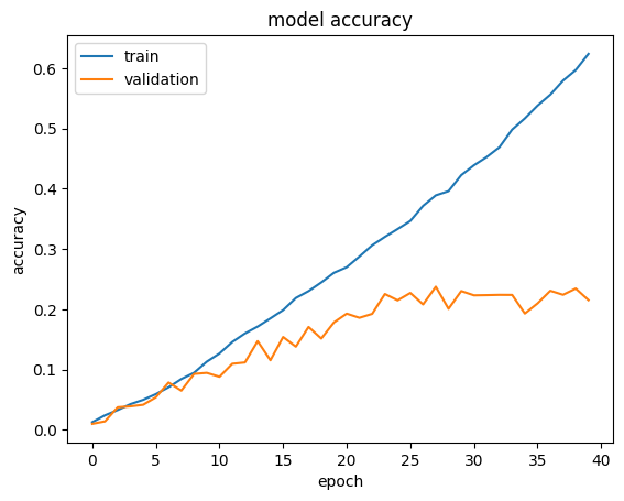
Training the model is relatively fast. This might make it sounds easy to simply train EfficientNet on any dataset wanted from scratch. However, training EfficientNet on smaller datasets, especially those with lower resolution like CIFAR-100, faces the significant challenge of overfitting.
Hence training from scratch requires very careful choice of hyperparameters and is difficult to find suitable regularization. It would also be much more demanding in resources. Plotting the training and validation accuracy makes it clear that validation accuracy stagnates at a low value.
import matplotlib.pyplot as plt


def plot_hist(hist):
    plt.plot(hist.history["accuracy"])
    plt.plot(hist.history["val_accuracy"])
    plt.title("model accuracy")
    plt.ylabel("accuracy")
    plt.xlabel("epoch")
    plt.legend(["train", "validation"], loc="upper left")
    plt.show()


plot_hist(hist)
Transfer learning from pre-trained weights
Here we initialize the model with pre-trained ImageNet weights, and we fine-tune it on our own dataset.
def build_model(num_classes):
    inputs = layers.Input(shape=(IMG_SIZE, IMG_SIZE, 3))
    model = EfficientNetB0(include_top=False, input_tensor=inputs, weights="imagenet")

    # Freeze the pretrained weights
    model.trainable = False

    # Rebuild top
    x = layers.GlobalAveragePooling2D(name="avg_pool")(model.output)
    x = layers.BatchNormalization()(x)

    top_dropout_rate = 0.2
    x = layers.Dropout(top_dropout_rate, name="top_dropout")(x)
    outputs = layers.Dense(num_classes, activation="softmax", name="pred")(x)

    # Compile
    model = keras.Model(inputs, outputs, name="EfficientNet")
    optimizer = keras.optimizers.Adam(learning_rate=1e-2)
    model.compile(
        optimizer=optimizer, loss="categorical_crossentropy", metrics=["accuracy"]
    )
    return model
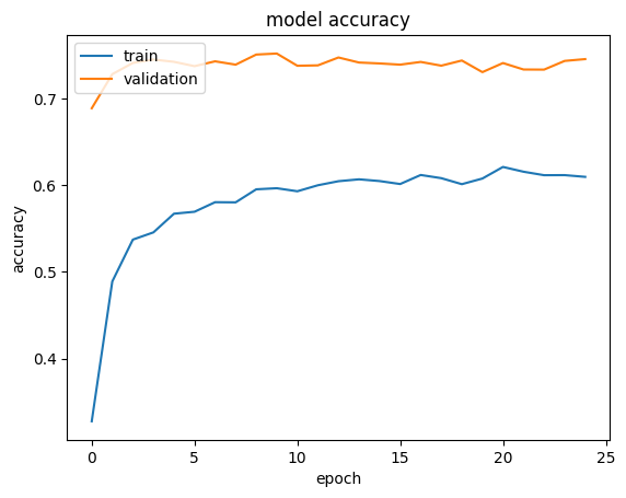
The first step to transfer learning is to freeze all layers and train only the top layers. For this step, a relatively large learning rate (1e-2) can be used. Note that validation accuracy and loss will usually be better than training accuracy and loss. This is because the regularization is strong, which only suppresses training-time metrics.
Note that the convergence may take up to 50 epochs depending on choice of learning rate. If image augmentation layers were not applied, the validation accuracy may only reach ~60%.
model = build_model(num_classes=NUM_CLASSES)

epochs = 25  # @param {type: "slider", min:8, max:80}
hist = model.fit(ds_train, epochs=epochs, validation_data=ds_test)
plot_hist(hist)
Epoch 1/25
 187/187 ━━━━━━━━━━━━━━━━━━━━ 108s 432ms/step - accuracy: 0.2654 - loss: 4.3710 - val_accuracy: 0.6888 - val_loss: 1.0875
Epoch 2/25
 187/187 ━━━━━━━━━━━━━━━━━━━━ 119s 412ms/step - accuracy: 0.4863 - loss: 2.0996 - val_accuracy: 0.7282 - val_loss: 0.9072
Epoch 3/25
 187/187 ━━━━━━━━━━━━━━━━━━━━ 78s 416ms/step - accuracy: 0.5422 - loss: 1.7120 - val_accuracy: 0.7411 - val_loss: 0.8574
Epoch 4/25
 187/187 ━━━━━━━━━━━━━━━━━━━━ 77s 412ms/step - accuracy: 0.5509 - loss: 1.6472 - val_accuracy: 0.7451 - val_loss: 0.8457
Epoch 5/25
 187/187 ━━━━━━━━━━━━━━━━━━━━ 81s 431ms/step - accuracy: 0.5744 - loss: 1.5373 - val_accuracy: 0.7424 - val_loss: 0.8649
Epoch 6/25
 187/187 ━━━━━━━━━━━━━━━━━━━━ 78s 417ms/step - accuracy: 0.5715 - loss: 1.5595 - val_accuracy: 0.7374 - val_loss: 0.8736
Epoch 7/25
 187/187 ━━━━━━━━━━━━━━━━━━━━ 81s 432ms/step - accuracy: 0.5802 - loss: 1.5045 - val_accuracy: 0.7430 - val_loss: 0.8675
Epoch 8/25
 187/187 ━━━━━━━━━━━━━━━━━━━━ 77s 411ms/step - accuracy: 0.5839 - loss: 1.4972 - val_accuracy: 0.7392 - val_loss: 0.8647
Epoch 9/25
 187/187 ━━━━━━━━━━━━━━━━━━━━ 77s 411ms/step - accuracy: 0.5929 - loss: 1.4699 - val_accuracy: 0.7508 - val_loss: 0.8634
Epoch 10/25
 187/187 ━━━━━━━━━━━━━━━━━━━━ 82s 437ms/step - accuracy: 0.6040 - loss: 1.4442 - val_accuracy: 0.7520 - val_loss: 0.8480
Epoch 11/25
 187/187 ━━━━━━━━━━━━━━━━━━━━ 78s 416ms/step - accuracy: 0.5972 - loss: 1.4626 - val_accuracy: 0.7379 - val_loss: 0.8879
Epoch 12/25
 187/187 ━━━━━━━━━━━━━━━━━━━━ 79s 421ms/step - accuracy: 0.5965 - loss: 1.4700 - val_accuracy: 0.7383 - val_loss: 0.9409
Epoch 13/25
 187/187 ━━━━━━━━━━━━━━━━━━━━ 82s 420ms/step - accuracy: 0.6034 - loss: 1.4533 - val_accuracy: 0.7474 - val_loss: 0.8922
Epoch 14/25
 187/187 ━━━━━━━━━━━━━━━━━━━━ 81s 435ms/step - accuracy: 0.6053 - loss: 1.4170 - val_accuracy: 0.7416 - val_loss: 0.9119
Epoch 15/25
 187/187 ━━━━━━━━━━━━━━━━━━━━ 77s 411ms/step - accuracy: 0.6059 - loss: 1.4125 - val_accuracy: 0.7406 - val_loss: 0.9205
Epoch 16/25
 187/187 ━━━━━━━━━━━━━━━━━━━━ 82s 438ms/step - accuracy: 0.5979 - loss: 1.4554 - val_accuracy: 0.7392 - val_loss: 0.9120
Epoch 17/25
 187/187 ━━━━━━━━━━━━━━━━━━━━ 77s 411ms/step - accuracy: 0.6081 - loss: 1.4089 - val_accuracy: 0.7423 - val_loss: 0.9305
Epoch 18/25
 187/187 ━━━━━━━━━━━━━━━━━━━━ 82s 436ms/step - accuracy: 0.6041 - loss: 1.4390 - val_accuracy: 0.7380 - val_loss: 0.9644
Epoch 19/25
 187/187 ━━━━━━━━━━━━━━━━━━━━ 79s 417ms/step - accuracy: 0.6018 - loss: 1.4324 - val_accuracy: 0.7439 - val_loss: 0.9129
Epoch 20/25
 187/187 ━━━━━━━━━━━━━━━━━━━━ 81s 430ms/step - accuracy: 0.6057 - loss: 1.4342 - val_accuracy: 0.7305 - val_loss: 0.9463
Epoch 21/25
 187/187 ━━━━━━━━━━━━━━━━━━━━ 77s 410ms/step - accuracy: 0.6209 - loss: 1.3824 - val_accuracy: 0.7410 - val_loss: 0.9503
Epoch 22/25
 187/187 ━━━━━━━━━━━━━━━━━━━━ 78s 419ms/step - accuracy: 0.6170 - loss: 1.4246 - val_accuracy: 0.7336 - val_loss: 0.9606
Epoch 23/25
 187/187 ━━━━━━━━━━━━━━━━━━━━ 85s 455ms/step - accuracy: 0.6153 - loss: 1.4009 - val_accuracy: 0.7334 - val_loss: 0.9520
Epoch 24/25
 187/187 ━━━━━━━━━━━━━━━━━━━━ 82s 438ms/step - accuracy: 0.6051 - loss: 1.4343 - val_accuracy: 0.7435 - val_loss: 0.9403
Epoch 25/25
 187/187 ━━━━━━━━━━━━━━━━━━━━ 138s 416ms/step - accuracy: 0.6065 - loss: 1.4131 - val_accuracy: 0.7456 - val_loss: 0.9307
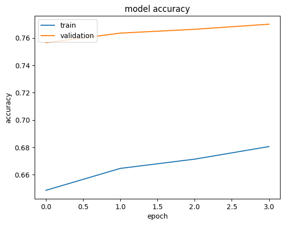
The second step is to unfreeze a number of layers and fit the model using smaller learning rate. In this example we show unfreezing all layers, but depending on specific dataset it may be desireble to only unfreeze a fraction of all layers.
When the feature extraction with pretrained model works good enough, this step would give a very limited gain on validation accuracy. In our case we only see a small improvement, as ImageNet pretraining already exposed the model to a good amount of dogs.
On the other hand, when we use pretrained weights on a dataset that is more different
from ImageNet, this fine-tuning step can be crucial as the feature extractor also
needs to be adjusted by a considerable amount. Such a situation can be demonstrated
if choosing CIFAR-100 dataset instead, where fine-tuning boosts validation accuracy
by about 10% to pass 80% on EfficientNetB0.
A side note on freezing/unfreezing models: setting trainable of a Model will
simultaneously set all layers belonging to the Model to the same trainable
attribute. Each layer is trainable only if both the layer itself and the model
containing it are trainable. Hence when we need to partially freeze/unfreeze
a model, we need to make sure the trainable attribute of the model is set
to True.
def unfreeze_model(model):
    # We unfreeze the top 20 layers while leaving BatchNorm layers frozen
    for layer in model.layers[-20:]:
        if not isinstance(layer, layers.BatchNormalization):
            layer.trainable = True

    optimizer = keras.optimizers.Adam(learning_rate=1e-5)
    model.compile(
        optimizer=optimizer, loss="categorical_crossentropy", metrics=["accuracy"]
    )


unfreeze_model(model)

epochs = 4  # @param {type: "slider", min:4, max:10}
hist = model.fit(ds_train, epochs=epochs, validation_data=ds_test)
plot_hist(hist)
Epoch 1/4
 187/187 ━━━━━━━━━━━━━━━━━━━━ 111s 442ms/step - accuracy: 0.6310 - loss: 1.3425 - val_accuracy: 0.7565 - val_loss: 0.8874
Epoch 2/4
 187/187 ━━━━━━━━━━━━━━━━━━━━ 77s 413ms/step - accuracy: 0.6518 - loss: 1.2755 - val_accuracy: 0.7635 - val_loss: 0.8588
Epoch 3/4
 187/187 ━━━━━━━━━━━━━━━━━━━━ 82s 437ms/step - accuracy: 0.6491 - loss: 1.2426 - val_accuracy: 0.7663 - val_loss: 0.8419
Epoch 4/4
 187/187 ━━━━━━━━━━━━━━━━━━━━ 79s 419ms/step - accuracy: 0.6625 - loss: 1.1775 - val_accuracy: 0.7701 - val_loss: 0.8284
Tips for fine tuning EfficientNet
On unfreezing layers:
- The
BatchNormalizationlayers need to be kept frozen (more details). If they are also turned to trainable, the first epoch after unfreezing will significantly reduce accuracy. - In some cases it may be beneficial to open up only a portion of layers instead of unfreezing all. This will make fine tuning much faster when going to larger models like B7.
- Each block needs to be all turned on or off. This is because the architecture includes a shortcut from the first layer to the last layer for each block. Not respecting blocks also significantly harms the final performance.
Some other tips for utilizing EfficientNet:
- Larger variants of EfficientNet do not guarantee improved performance, especially for tasks with less data or fewer classes. In such a case, the larger variant of EfficientNet chosen, the harder it is to tune hyperparameters.
- EMA (Exponential Moving Average) is very helpful in training EfficientNet from scratch, but not so much for transfer learning.
- Do not use the RMSprop setup as in the original paper for transfer learning. The momentum and learning rate are too high for transfer learning. It will easily corrupt the pretrained weight and blow up the loss. A quick check is to see if loss (as categorical cross entropy) is getting significantly larger than log(NUM_CLASSES) after the same epoch. If so, the initial learning rate/momentum is too high.
- Smaller batch size benefit validation accuracy, possibly due to effectively providing regularization.