Using the Forward-Forward Algorithm for Image Classification
Author: Suvaditya Mukherjee
Date created: 2023/01/08
Last modified: 2024/09/17
Description: Training a Dense-layer model using the Forward-Forward algorithm.

Introduction
The following example explores how to use the Forward-Forward algorithm to perform training instead of the traditionally-used method of backpropagation, as proposed by Hinton in The Forward-Forward Algorithm: Some Preliminary Investigations (2022).
The concept was inspired by the understanding behind Boltzmann Machines. Backpropagation involves calculating the difference between actual and predicted output via a cost function to adjust network weights. On the other hand, the FF Algorithm suggests the analogy of neurons which get "excited" based on looking at a certain recognized combination of an image and its correct corresponding label.
This method takes certain inspiration from the biological learning process that occurs in the cortex. A significant advantage that this method brings is the fact that backpropagation through the network does not need to be performed anymore, and that weight updates are local to the layer itself.
As this is yet still an experimental method, it does not yield state-of-the-art results. But with proper tuning, it is supposed to come close to the same. Through this example, we will examine a process that allows us to implement the Forward-Forward algorithm within the layers themselves, instead of the traditional method of relying on the global loss functions and optimizers.
The tutorial is structured as follows:
- Perform necessary imports
- Load the MNIST dataset
- Visualize Random samples from the MNIST dataset
- Define a
FFDenseLayer to overridecalland implement a customforwardforwardmethod which performs weight updates. - Define a
FFNetworkLayer to overridetrain_step,predictand implement 2 custom functions for per-sample prediction and overlaying labels - Convert MNIST from
NumPyarrays totf.data.Dataset - Fit the network
- Visualize results
- Perform inference on test samples
As this example requires the customization of certain core functions with
keras.layers.Layer and keras.models.Model, refer to the following resources for
a primer on how to do so:
Setup imports
import os

os.environ["KERAS_BACKEND"] = "tensorflow"

import tensorflow as tf
import keras
from keras import ops
import numpy as np
import matplotlib.pyplot as plt
from sklearn.metrics import accuracy_score
import random
from tensorflow.compiler.tf2xla.python import xla
Load the dataset and visualize the data
We use the keras.datasets.mnist.load_data() utility to directly pull the MNIST dataset
in the form of NumPy arrays. We then arrange it in the form of the train and test
splits.
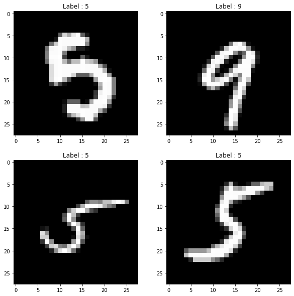
Following loading the dataset, we select 4 random samples from within the training set
and visualize them using matplotlib.pyplot.
(x_train, y_train), (x_test, y_test) = keras.datasets.mnist.load_data()

print("4 Random Training samples and labels")
idx1, idx2, idx3, idx4 = random.sample(range(0, x_train.shape[0]), 4)

img1 = (x_train[idx1], y_train[idx1])
img2 = (x_train[idx2], y_train[idx2])
img3 = (x_train[idx3], y_train[idx3])
img4 = (x_train[idx4], y_train[idx4])

imgs = [img1, img2, img3, img4]

plt.figure(figsize=(10, 10))

for idx, item in enumerate(imgs):
    image, label = item[0], item[1]
    plt.subplot(2, 2, idx + 1)
    plt.imshow(image, cmap="gray")
    plt.title(f"Label : {label}")
plt.show()
4 Random Training samples and labels
Define FFDense custom layer
In this custom layer, we have a base keras.layers.Dense object which acts as the
base Dense layer within. Since weight updates will happen within the layer itself, we
add an keras.optimizers.Optimizer object that is accepted from the user. Here, we
use Adam as our optimizer with a rather higher learning rate of 0.03.
Following the algorithm's specifics, we must set a threshold parameter that will be
used to make the positive-negative decision in each prediction. This is set to a default
of 2.0.
As the epochs are localized to the layer itself, we also set a num_epochs parameter
(defaults to 50).
We override the call method in order to perform a normalization over the complete
input space followed by running it through the base Dense layer as would happen in a
normal Dense layer call.
We implement the Forward-Forward algorithm which accepts 2 kinds of input tensors, each
representing the positive and negative samples respectively. We write a custom training
loop here with the use of tf.GradientTape(), within which we calculate a loss per
sample by taking the distance of the prediction from the threshold to understand the
error and taking its mean to get a mean_loss metric.
With the help of tf.GradientTape() we calculate the gradient updates for the trainable
base Dense layer and apply them using the layer's local optimizer.
Finally, we return the call result as the Dense results of the positive and negative
samples while also returning the last mean_loss metric and all the loss values over a
certain all-epoch run.
class FFDense(keras.layers.Layer):
    """
    A custom ForwardForward-enabled Dense layer. It has an implementation of the
    Forward-Forward network internally for use.
    This layer must be used in conjunction with the `FFNetwork` model.
    """

    def __init__(
        self,
        units,
        init_optimizer,
        loss_metric,
        num_epochs=50,
        use_bias=True,
        kernel_initializer="glorot_uniform",
        bias_initializer="zeros",
        kernel_regularizer=None,
        bias_regularizer=None,
        **kwargs,
    ):
        super().__init__(**kwargs)
        self.dense = keras.layers.Dense(
            units=units,
            use_bias=use_bias,
            kernel_initializer=kernel_initializer,
            bias_initializer=bias_initializer,
            kernel_regularizer=kernel_regularizer,
            bias_regularizer=bias_regularizer,
        )
        self.relu = keras.layers.ReLU()
        self.optimizer = init_optimizer()
        self.loss_metric = loss_metric
        self.threshold = 1.5
        self.num_epochs = num_epochs

    # We perform a normalization step before we run the input through the Dense
    # layer.

    def call(self, x):
        x_norm = ops.norm(x, ord=2, axis=1, keepdims=True)
        x_norm = x_norm + 1e-4
        x_dir = x / x_norm
        res = self.dense(x_dir)
        return self.relu(res)

    # The Forward-Forward algorithm is below. We first perform the Dense-layer
    # operation and then get a Mean Square value for all positive and negative
    # samples respectively.
    # The custom loss function finds the distance between the Mean-squared
    # result and the threshold value we set (a hyperparameter) that will define
    # whether the prediction is positive or negative in nature. Once the loss is
    # calculated, we get a mean across the entire batch combined and perform a
    # gradient calculation and optimization step. This does not technically
    # qualify as backpropagation since there is no gradient being
    # sent to any previous layer and is completely local in nature.

    def forward_forward(self, x_pos, x_neg):
        for i in range(self.num_epochs):
            with tf.GradientTape() as tape:
                g_pos = ops.mean(ops.power(self.call(x_pos), 2), 1)
                g_neg = ops.mean(ops.power(self.call(x_neg), 2), 1)

                loss = ops.log(
                    1
                    + ops.exp(
                        ops.concatenate(
                            [-g_pos + self.threshold, g_neg - self.threshold], 0
                        )
                    )
                )
                mean_loss = ops.cast(ops.mean(loss), dtype="float32")
                self.loss_metric.update_state([mean_loss])
            gradients = tape.gradient(mean_loss, self.dense.trainable_weights)
            self.optimizer.apply_gradients(zip(gradients, self.dense.trainable_weights))
        return (
            ops.stop_gradient(self.call(x_pos)),
            ops.stop_gradient(self.call(x_neg)),
            self.loss_metric.result(),
        )
Define the FFNetwork Custom Model
With our custom layer defined, we also need to override the train_step method and
define a custom keras.models.Model that works with our FFDense layer.
For this algorithm, we must 'embed' the labels onto the original image. To do so, we
exploit the structure of MNIST images where the top-left 10 pixels are always zeros. We
use that as a label space in order to visually one-hot-encode the labels within the image
itself. This action is performed by the overlay_y_on_x function.
We break down the prediction function with a per-sample prediction function which is then
called over the entire test set by the overriden predict() function. The prediction is
performed here with the help of measuring the excitation of the neurons per layer for
each image. This is then summed over all layers to calculate a network-wide 'goodness
score'. The label with the highest 'goodness score' is then chosen as the sample
prediction.
The train_step function is overriden to act as the main controlling loop for running
training on each layer as per the number of epochs per layer.
class FFNetwork(keras.Model):
    """
    A [`keras.Model`](/api/models/model#model-class) that supports a `FFDense` network creation. This model
    can work for any kind of classification task. It has an internal
    implementation with some details specific to the MNIST dataset which can be
    changed as per the use-case.
    """

    # Since each layer runs gradient-calculation and optimization locally, each
    # layer has its own optimizer that we pass. As a standard choice, we pass
    # the `Adam` optimizer with a default learning rate of 0.03 as that was
    # found to be the best rate after experimentation.
    # Loss is tracked using `loss_var` and `loss_count` variables.

    def __init__(
        self,
        dims,
        init_layer_optimizer=lambda: keras.optimizers.Adam(learning_rate=0.03),
        **kwargs,
    ):
        super().__init__(**kwargs)
        self.init_layer_optimizer = init_layer_optimizer
        self.loss_var = keras.Variable(0.0, trainable=False, dtype="float32")
        self.loss_count = keras.Variable(0.0, trainable=False, dtype="float32")
        self.layer_list = [keras.Input(shape=(dims[0],))]
        self.metrics_built = False
        for d in range(len(dims) - 1):
            self.layer_list += [
                FFDense(
                    dims[d + 1],
                    init_optimizer=self.init_layer_optimizer,
                    loss_metric=keras.metrics.Mean(),
                )
            ]

    # This function makes a dynamic change to the image wherein the labels are
    # put on top of the original image (for this example, as MNIST has 10
    # unique labels, we take the top-left corner's first 10 pixels). This
    # function returns the original data tensor with the first 10 pixels being
    # a pixel-based one-hot representation of the labels.

    @tf.function(reduce_retracing=True)
    def overlay_y_on_x(self, data):
        X_sample, y_sample = data
        max_sample = ops.amax(X_sample, axis=0, keepdims=True)
        max_sample = ops.cast(max_sample, dtype="float64")
        X_zeros = ops.zeros([10], dtype="float64")
        X_update = xla.dynamic_update_slice(X_zeros, max_sample, [y_sample])
        X_sample = xla.dynamic_update_slice(X_sample, X_update, [0])
        return X_sample, y_sample

    # A custom `predict_one_sample` performs predictions by passing the images
    # through the network, measures the results produced by each layer (i.e.
    # how high/low the output values are with respect to the set threshold for
    # each label) and then simply finding the label with the highest values.
    # In such a case, the images are tested for their 'goodness' with all
    # labels.

    @tf.function(reduce_retracing=True)
    def predict_one_sample(self, x):
        goodness_per_label = []
        x = ops.reshape(x, [ops.shape(x)[0] * ops.shape(x)[1]])
        for label in range(10):
            h, label = self.overlay_y_on_x(data=(x, label))
            h = ops.reshape(h, [-1, ops.shape(h)[0]])
            goodness = []
            for layer_idx in range(1, len(self.layer_list)):
                layer = self.layer_list[layer_idx]
                h = layer(h)
                goodness += [ops.mean(ops.power(h, 2), 1)]
            goodness_per_label += [ops.expand_dims(ops.sum(goodness, keepdims=True), 1)]
        goodness_per_label = tf.concat(goodness_per_label, 1)
        return ops.cast(ops.argmax(goodness_per_label, 1), dtype="float64")

    def predict(self, data):
        x = data
        preds = list()
        preds = ops.vectorized_map(self.predict_one_sample, x)
        return np.asarray(preds, dtype=int)

    # This custom `train_step` function overrides the internal `train_step`
    # implementation. We take all the input image tensors, flatten them and
    # subsequently produce positive and negative samples on the images.
    # A positive sample is an image that has the right label encoded on it with
    # the `overlay_y_on_x` function. A negative sample is an image that has an
    # erroneous label present on it.
    # With the samples ready, we pass them through each `FFLayer` and perform
    # the Forward-Forward computation on it. The returned loss is the final
    # loss value over all the layers.

    @tf.function(jit_compile=False)
    def train_step(self, data):
        x, y = data

        if not self.metrics_built:
            # build metrics to ensure they can be queried without erroring out.
            # We can't update the metrics' state, as we would usually do, since
            # we do not perform predictions within the train step
            for metric in self.metrics:
                if hasattr(metric, "build"):
                    metric.build(y, y)
            self.metrics_built = True

        # Flatten op
        x = ops.reshape(x, [-1, ops.shape(x)[1] * ops.shape(x)[2]])

        x_pos, y = ops.vectorized_map(self.overlay_y_on_x, (x, y))

        random_y = tf.random.shuffle(y)
        x_neg, y = tf.map_fn(self.overlay_y_on_x, (x, random_y))

        h_pos, h_neg = x_pos, x_neg

        for idx, layer in enumerate(self.layers):
            if isinstance(layer, FFDense):
                print(f"Training layer {idx+1} now : ")
                h_pos, h_neg, loss = layer.forward_forward(h_pos, h_neg)
                self.loss_var.assign_add(loss)
                self.loss_count.assign_add(1.0)
            else:
                print(f"Passing layer {idx+1} now : ")
                x = layer(x)
        mean_res = ops.divide(self.loss_var, self.loss_count)
        return {"FinalLoss": mean_res}
Convert MNIST NumPy arrays to tf.data.Dataset
We now perform some preliminary processing on the NumPy arrays and then convert them
into the tf.data.Dataset format which allows for optimized loading.
x_train = x_train.astype(float) / 255
x_test = x_test.astype(float) / 255
y_train = y_train.astype(int)
y_test = y_test.astype(int)

train_dataset = tf.data.Dataset.from_tensor_slices((x_train, y_train))
test_dataset = tf.data.Dataset.from_tensor_slices((x_test, y_test))

train_dataset = train_dataset.batch(60000)
test_dataset = test_dataset.batch(10000)
Fit the network and visualize results
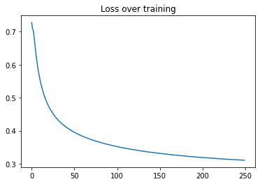
Having performed all previous set-up, we are now going to run model.fit() and run 250
model epochs, which will perform 50*250 epochs on each layer. We get to see the plotted loss
curve as each layer is trained.
model = FFNetwork(dims=[784, 500, 500])

model.compile(
    optimizer=keras.optimizers.Adam(learning_rate=0.03),
    loss="mse",
    jit_compile=False,
    metrics=[],
)

epochs = 250
history = model.fit(train_dataset, epochs=epochs)
Epoch 1/250

Training layer 1 now :

Training layer 2 now :

Training layer 1 now :

Training layer 2 now :
1/1 ━━━━━━━━━━━━━━━━━━━━ 90s 90s/step - FinalLoss: 0.7247

Epoch 2/250
1/1 ━━━━━━━━━━━━━━━━━━━━ 41s 41s/step - FinalLoss: 0.7089

Epoch 3/250
 1/1 ━━━━━━━━━━━━━━━━━━━━ 41s 41s/step - FinalLoss: 0.6978

Epoch 4/250
1/1 ━━━━━━━━━━━━━━━━━━━━ 40s 40s/step - FinalLoss: 0.6827

Epoch 5/250
1/1 ━━━━━━━━━━━━━━━━━━━━ 40s 40s/step - FinalLoss: 0.6644

Epoch 6/250
1/1 ━━━━━━━━━━━━━━━━━━━━ 40s 40s/step - FinalLoss: 0.6462

Epoch 7/250
1/1 ━━━━━━━━━━━━━━━━━━━━ 40s 40s/step - FinalLoss: 0.6290

Epoch 8/250
1/1 ━━━━━━━━━━━━━━━━━━━━ 40s 40s/step - FinalLoss: 0.6131

Epoch 9/250
1/1 ━━━━━━━━━━━━━━━━━━━━ 40s 40s/step - FinalLoss: 0.5986

Epoch 10/250
1/1 ━━━━━━━━━━━━━━━━━━━━ 40s 40s/step - FinalLoss: 0.5853

Epoch 11/250
1/1 ━━━━━━━━━━━━━━━━━━━━ 40s 40s/step - FinalLoss: 0.5731

Epoch 12/250
1/1 ━━━━━━━━━━━━━━━━━━━━ 40s 40s/step - FinalLoss: 0.5621

Epoch 13/250
1/1 ━━━━━━━━━━━━━━━━━━━━ 40s 40s/step - FinalLoss: 0.5519

Epoch 14/250
1/1 ━━━━━━━━━━━━━━━━━━━━ 40s 40s/step - FinalLoss: 0.5425

Epoch 15/250
1/1 ━━━━━━━━━━━━━━━━━━━━ 40s 40s/step - FinalLoss: 0.5338

Epoch 16/250
1/1 ━━━━━━━━━━━━━━━━━━━━ 40s 40s/step - FinalLoss: 0.5259

Epoch 17/250
1/1 ━━━━━━━━━━━━━━━━━━━━ 40s 40s/step - FinalLoss: 0.5186

Epoch 18/250
1/1 ━━━━━━━━━━━━━━━━━━━━ 40s 40s/step - FinalLoss: 0.5117

Epoch 19/250
1/1 ━━━━━━━━━━━━━━━━━━━━ 40s 40s/step - FinalLoss: 0.5052

Epoch 20/250
1/1 ━━━━━━━━━━━━━━━━━━━━ 40s 40s/step - FinalLoss: 0.4992

Epoch 21/250
1/1 ━━━━━━━━━━━━━━━━━━━━ 40s 40s/step - FinalLoss: 0.4935

Epoch 22/250
1/1 ━━━━━━━━━━━━━━━━━━━━ 40s 40s/step - FinalLoss: 0.4883

Epoch 23/250
1/1 ━━━━━━━━━━━━━━━━━━━━ 40s 40s/step - FinalLoss: 0.4833

Epoch 24/250
1/1 ━━━━━━━━━━━━━━━━━━━━ 40s 40s/step - FinalLoss: 0.4786

Epoch 25/250
1/1 ━━━━━━━━━━━━━━━━━━━━ 40s 40s/step - FinalLoss: 0.4741

Epoch 26/250
1/1 ━━━━━━━━━━━━━━━━━━━━ 41s 41s/step - FinalLoss: 0.4698

Epoch 27/250
1/1 ━━━━━━━━━━━━━━━━━━━━ 41s 41s/step - FinalLoss: 0.4658

Epoch 28/250
1/1 ━━━━━━━━━━━━━━━━━━━━ 41s 41s/step - FinalLoss: 0.4620

Epoch 29/250
1/1 ━━━━━━━━━━━━━━━━━━━━ 40s 40s/step - FinalLoss: 0.4584

Epoch 30/250
1/1 ━━━━━━━━━━━━━━━━━━━━ 41s 41s/step - FinalLoss: 0.4550

Epoch 31/250
1/1 ━━━━━━━━━━━━━━━━━━━━ 41s 41s/step - FinalLoss: 0.4517

Epoch 32/250
1/1 ━━━━━━━━━━━━━━━━━━━━ 41s 41s/step - FinalLoss: 0.4486

Epoch 33/250
1/1 ━━━━━━━━━━━━━━━━━━━━ 41s 41s/step - FinalLoss: 0.4456

Epoch 34/250
1/1 ━━━━━━━━━━━━━━━━━━━━ 41s 41s/step - FinalLoss: 0.4429

Epoch 35/250
1/1 ━━━━━━━━━━━━━━━━━━━━ 41s 41s/step - FinalLoss: 0.4401

Epoch 36/250
1/1 ━━━━━━━━━━━━━━━━━━━━ 41s 41s/step - FinalLoss: 0.4375

Epoch 37/250
1/1 ━━━━━━━━━━━━━━━━━━━━ 41s 41s/step - FinalLoss: 0.4350

Epoch 38/250
1/1 ━━━━━━━━━━━━━━━━━━━━ 41s 41s/step - FinalLoss: 0.4325

Epoch 39/250
1/1 ━━━━━━━━━━━━━━━━━━━━ 41s 41s/step - FinalLoss: 0.4302

Epoch 40/250
1/1 ━━━━━━━━━━━━━━━━━━━━ 41s 41s/step - FinalLoss: 0.4279

Epoch 41/250
1/1 ━━━━━━━━━━━━━━━━━━━━ 41s 41s/step - FinalLoss: 0.4258

Epoch 42/250
1/1 ━━━━━━━━━━━━━━━━━━━━ 41s 41s/step - FinalLoss: 0.4236

Epoch 43/250
1/1 ━━━━━━━━━━━━━━━━━━━━ 41s 41s/step - FinalLoss: 0.4216

Epoch 44/250
1/1 ━━━━━━━━━━━━━━━━━━━━ 41s 41s/step - FinalLoss: 0.4197

Epoch 45/250
1/1 ━━━━━━━━━━━━━━━━━━━━ 41s 41s/step - FinalLoss: 0.4177

Epoch 46/250
1/1 ━━━━━━━━━━━━━━━━━━━━ 41s 41s/step - FinalLoss: 0.4159

Epoch 47/250
1/1 ━━━━━━━━━━━━━━━━━━━━ 41s 41s/step - FinalLoss: 0.4141

Epoch 48/250
1/1 ━━━━━━━━━━━━━━━━━━━━ 40s 40s/step - FinalLoss: 0.4124

Epoch 49/250
1/1 ━━━━━━━━━━━━━━━━━━━━ 40s 40s/step - FinalLoss: 0.4107

Epoch 50/250
1/1 ━━━━━━━━━━━━━━━━━━━━ 40s 40s/step - FinalLoss: 0.4090

Epoch 51/250
1/1 ━━━━━━━━━━━━━━━━━━━━ 40s 40s/step - FinalLoss: 0.4074

Epoch 52/250
1/1 ━━━━━━━━━━━━━━━━━━━━ 40s 40s/step - FinalLoss: 0.4059

Epoch 53/250
1/1 ━━━━━━━━━━━━━━━━━━━━ 40s 40s/step - FinalLoss: 0.4044

Epoch 54/250
1/1 ━━━━━━━━━━━━━━━━━━━━ 40s 40s/step - FinalLoss: 0.4030

Epoch 55/250
1/1 ━━━━━━━━━━━━━━━━━━━━ 41s 41s/step - FinalLoss: 0.4016

Epoch 56/250
1/1 ━━━━━━━━━━━━━━━━━━━━ 41s 41s/step - FinalLoss: 0.4002

Epoch 57/250
1/1 ━━━━━━━━━━━━━━━━━━━━ 41s 41s/step - FinalLoss: 0.3988

Epoch 58/250
1/1 ━━━━━━━━━━━━━━━━━━━━ 41s 41s/step - FinalLoss: 0.3975

Epoch 59/250
1/1 ━━━━━━━━━━━━━━━━━━━━ 40s 40s/step - FinalLoss: 0.3962

Epoch 60/250
1/1 ━━━━━━━━━━━━━━━━━━━━ 40s 40s/step - FinalLoss: 0.3950

Epoch 61/250
1/1 ━━━━━━━━━━━━━━━━━━━━ 40s 40s/step - FinalLoss: 0.3938

Epoch 62/250
1/1 ━━━━━━━━━━━━━━━━━━━━ 40s 40s/step - FinalLoss: 0.3926

Epoch 63/250
1/1 ━━━━━━━━━━━━━━━━━━━━ 40s 40s/step - FinalLoss: 0.3914

Epoch 64/250
1/1 ━━━━━━━━━━━━━━━━━━━━ 40s 40s/step - FinalLoss: 0.3903

Epoch 65/250
1/1 ━━━━━━━━━━━━━━━━━━━━ 40s 40s/step - FinalLoss: 0.3891

Epoch 66/250
1/1 ━━━━━━━━━━━━━━━━━━━━ 40s 40s/step - FinalLoss: 0.3880

Epoch 67/250
1/1 ━━━━━━━━━━━━━━━━━━━━ 40s 40s/step - FinalLoss: 0.3869

Epoch 68/250
1/1 ━━━━━━━━━━━━━━━━━━━━ 40s 40s/step - FinalLoss: 0.3859

Epoch 69/250
1/1 ━━━━━━━━━━━━━━━━━━━━ 40s 40s/step - FinalLoss: 0.3849

Epoch 70/250
1/1 ━━━━━━━━━━━━━━━━━━━━ 41s 41s/step - FinalLoss: 0.3839

Epoch 71/250
1/1 ━━━━━━━━━━━━━━━━━━━━ 41s 41s/step - FinalLoss: 0.3829

Epoch 72/250
1/1 ━━━━━━━━━━━━━━━━━━━━ 41s 41s/step - FinalLoss: 0.3819

Epoch 73/250
1/1 ━━━━━━━━━━━━━━━━━━━━ 41s 41s/step - FinalLoss: 0.3810

Epoch 74/250
1/1 ━━━━━━━━━━━━━━━━━━━━ 41s 41s/step - FinalLoss: 0.3801

Epoch 75/250
1/1 ━━━━━━━━━━━━━━━━━━━━ 41s 41s/step - FinalLoss: 0.3792

Epoch 76/250
1/1 ━━━━━━━━━━━━━━━━━━━━ 41s 41s/step - FinalLoss: 0.3783

Epoch 77/250
1/1 ━━━━━━━━━━━━━━━━━━━━ 41s 41s/step - FinalLoss: 0.3774

Epoch 78/250
1/1 ━━━━━━━━━━━━━━━━━━━━ 41s 41s/step - FinalLoss: 0.3765

Epoch 79/250
1/1 ━━━━━━━━━━━━━━━━━━━━ 41s 41s/step - FinalLoss: 0.3757

Epoch 80/250
1/1 ━━━━━━━━━━━━━━━━━━━━ 41s 41s/step - FinalLoss: 0.3748

Epoch 81/250
1/1 ━━━━━━━━━━━━━━━━━━━━ 41s 41s/step - FinalLoss: 0.3740

Epoch 82/250
1/1 ━━━━━━━━━━━━━━━━━━━━ 41s 41s/step - FinalLoss: 0.3732

Epoch 83/250
1/1 ━━━━━━━━━━━━━━━━━━━━ 41s 41s/step - FinalLoss: 0.3723

Epoch 84/250
1/1 ━━━━━━━━━━━━━━━━━━━━ 41s 41s/step - FinalLoss: 0.3715

Epoch 85/250
1/1 ━━━━━━━━━━━━━━━━━━━━ 41s 41s/step - FinalLoss: 0.3708

Epoch 86/250
1/1 ━━━━━━━━━━━━━━━━━━━━ 41s 41s/step - FinalLoss: 0.3700

Epoch 87/250
1/1 ━━━━━━━━━━━━━━━━━━━━ 41s 41s/step - FinalLoss: 0.3692

Epoch 88/250
1/1 ━━━━━━━━━━━━━━━━━━━━ 41s 41s/step - FinalLoss: 0.3685

Epoch 89/250
1/1 ━━━━━━━━━━━━━━━━━━━━ 41s 41s/step - FinalLoss: 0.3677

Epoch 90/250
1/1 ━━━━━━━━━━━━━━━━━━━━ 41s 41s/step - FinalLoss: 0.3670

Epoch 91/250
1/1 ━━━━━━━━━━━━━━━━━━━━ 41s 41s/step - FinalLoss: 0.3663

Epoch 92/250
1/1 ━━━━━━━━━━━━━━━━━━━━ 41s 41s/step - FinalLoss: 0.3656

Epoch 93/250
1/1 ━━━━━━━━━━━━━━━━━━━━ 40s 40s/step - FinalLoss: 0.3649

Epoch 94/250
1/1 ━━━━━━━━━━━━━━━━━━━━ 40s 40s/step - FinalLoss: 0.3642

Epoch 95/250
1/1 ━━━━━━━━━━━━━━━━━━━━ 41s 41s/step - FinalLoss: 0.3635

Epoch 96/250
1/1 ━━━━━━━━━━━━━━━━━━━━ 41s 41s/step - FinalLoss: 0.3629

Epoch 97/250
1/1 ━━━━━━━━━━━━━━━━━━━━ 40s 40s/step - FinalLoss: 0.3622

Epoch 98/250
1/1 ━━━━━━━━━━━━━━━━━━━━ 40s 40s/step - FinalLoss: 0.3616

Epoch 99/250
1/1 ━━━━━━━━━━━━━━━━━━━━ 40s 40s/step - FinalLoss: 0.3610

Epoch 100/250
1/1 ━━━━━━━━━━━━━━━━━━━━ 40s 40s/step - FinalLoss: 0.3603

Epoch 101/250
1/1 ━━━━━━━━━━━━━━━━━━━━ 40s 40s/step - FinalLoss: 0.3597

Epoch 102/250
1/1 ━━━━━━━━━━━━━━━━━━━━ 40s 40s/step - FinalLoss: 0.3591

Epoch 103/250
1/1 ━━━━━━━━━━━━━━━━━━━━ 40s 40s/step - FinalLoss: 0.3585

Epoch 104/250
1/1 ━━━━━━━━━━━━━━━━━━━━ 40s 40s/step - FinalLoss: 0.3579

Epoch 105/250
1/1 ━━━━━━━━━━━━━━━━━━━━ 40s 40s/step - FinalLoss: 0.3573

Epoch 106/250
1/1 ━━━━━━━━━━━━━━━━━━━━ 40s 40s/step - FinalLoss: 0.3567

Epoch 107/250
1/1 ━━━━━━━━━━━━━━━━━━━━ 40s 40s/step - FinalLoss: 0.3562

Epoch 108/250
1/1 ━━━━━━━━━━━━━━━━━━━━ 40s 40s/step - FinalLoss: 0.3556

Epoch 109/250
1/1 ━━━━━━━━━━━━━━━━━━━━ 40s 40s/step - FinalLoss: 0.3550

Epoch 110/250
1/1 ━━━━━━━━━━━━━━━━━━━━ 40s 40s/step - FinalLoss: 0.3545

Epoch 111/250
1/1 ━━━━━━━━━━━━━━━━━━━━ 40s 40s/step - FinalLoss: 0.3539

Epoch 112/250
1/1 ━━━━━━━━━━━━━━━━━━━━ 40s 40s/step - FinalLoss: 0.3534

Epoch 113/250
1/1 ━━━━━━━━━━━━━━━━━━━━ 40s 40s/step - FinalLoss: 0.3529

Epoch 114/250
1/1 ━━━━━━━━━━━━━━━━━━━━ 40s 40s/step - FinalLoss: 0.3524

Epoch 115/250
1/1 ━━━━━━━━━━━━━━━━━━━━ 40s 40s/step - FinalLoss: 0.3519

Epoch 116/250
1/1 ━━━━━━━━━━━━━━━━━━━━ 41s 41s/step - FinalLoss: 0.3513

Epoch 117/250
1/1 ━━━━━━━━━━━━━━━━━━━━ 41s 41s/step - FinalLoss: 0.3508

Epoch 118/250
1/1 ━━━━━━━━━━━━━━━━━━━━ 41s 41s/step - FinalLoss: 0.3503

Epoch 119/250
1/1 ━━━━━━━━━━━━━━━━━━━━ 41s 41s/step - FinalLoss: 0.3498

Epoch 120/250
1/1 ━━━━━━━━━━━━━━━━━━━━ 41s 41s/step - FinalLoss: 0.3493

Epoch 121/250
1/1 ━━━━━━━━━━━━━━━━━━━━ 41s 41s/step - FinalLoss: 0.3488

Epoch 122/250
1/1 ━━━━━━━━━━━━━━━━━━━━ 41s 41s/step - FinalLoss: 0.3484

Epoch 123/250
1/1 ━━━━━━━━━━━━━━━━━━━━ 41s 41s/step - FinalLoss: 0.3479

Epoch 124/250
1/1 ━━━━━━━━━━━━━━━━━━━━ 41s 41s/step - FinalLoss: 0.3474

Epoch 125/250
1/1 ━━━━━━━━━━━━━━━━━━━━ 41s 41s/step - FinalLoss: 0.3470

Epoch 126/250
1/1 ━━━━━━━━━━━━━━━━━━━━ 41s 41s/step - FinalLoss: 0.3465

Epoch 127/250
1/1 ━━━━━━━━━━━━━━━━━━━━ 41s 41s/step - FinalLoss: 0.3461

Epoch 128/250
1/1 ━━━━━━━━━━━━━━━━━━━━ 41s 41s/step - FinalLoss: 0.3456

Epoch 129/250
1/1 ━━━━━━━━━━━━━━━━━━━━ 41s 41s/step - FinalLoss: 0.3452

Epoch 130/250
1/1 ━━━━━━━━━━━━━━━━━━━━ 41s 41s/step - FinalLoss: 0.3447

Epoch 131/250
1/1 ━━━━━━━━━━━━━━━━━━━━ 41s 41s/step - FinalLoss: 0.3443

Epoch 132/250
1/1 ━━━━━━━━━━━━━━━━━━━━ 41s 41s/step - FinalLoss: 0.3439

Epoch 133/250
1/1 ━━━━━━━━━━━━━━━━━━━━ 41s 41s/step - FinalLoss: 0.3435

Epoch 134/250
1/1 ━━━━━━━━━━━━━━━━━━━━ 41s 41s/step - FinalLoss: 0.3430

Epoch 135/250
1/1 ━━━━━━━━━━━━━━━━━━━━ 41s 41s/step - FinalLoss: 0.3426

Epoch 136/250
1/1 ━━━━━━━━━━━━━━━━━━━━ 41s 41s/step - FinalLoss: 0.3422

Epoch 137/250
1/1 ━━━━━━━━━━━━━━━━━━━━ 40s 40s/step - FinalLoss: 0.3418

Epoch 138/250
1/1 ━━━━━━━━━━━━━━━━━━━━ 41s 41s/step - FinalLoss: 0.3414

Epoch 139/250
1/1 ━━━━━━━━━━━━━━━━━━━━ 40s 40s/step - FinalLoss: 0.3411

Epoch 140/250
1/1 ━━━━━━━━━━━━━━━━━━━━ 40s 40s/step - FinalLoss: 0.3407

Epoch 141/250
1/1 ━━━━━━━━━━━━━━━━━━━━ 40s 40s/step - FinalLoss: 0.3403

Epoch 142/250
1/1 ━━━━━━━━━━━━━━━━━━━━ 40s 40s/step - FinalLoss: 0.3399

Epoch 143/250
1/1 ━━━━━━━━━━━━━━━━━━━━ 40s 40s/step - FinalLoss: 0.3395

Epoch 144/250
1/1 ━━━━━━━━━━━━━━━━━━━━ 40s 40s/step - FinalLoss: 0.3391

Epoch 145/250
1/1 ━━━━━━━━━━━━━━━━━━━━ 41s 41s/step - FinalLoss: 0.3387

Epoch 146/250
1/1 ━━━━━━━━━━━━━━━━━━━━ 40s 40s/step - FinalLoss: 0.3384

Epoch 147/250
1/1 ━━━━━━━━━━━━━━━━━━━━ 40s 40s/step - FinalLoss: 0.3380

Epoch 148/250
1/1 ━━━━━━━━━━━━━━━━━━━━ 40s 40s/step - FinalLoss: 0.3376

Epoch 149/250
1/1 ━━━━━━━━━━━━━━━━━━━━ 40s 40s/step - FinalLoss: 0.3373

Epoch 150/250
1/1 ━━━━━━━━━━━━━━━━━━━━ 40s 40s/step - FinalLoss: 0.3369

Epoch 151/250
1/1 ━━━━━━━━━━━━━━━━━━━━ 40s 40s/step - FinalLoss: 0.3366

Epoch 152/250
1/1 ━━━━━━━━━━━━━━━━━━━━ 41s 41s/step - FinalLoss: 0.3362

Epoch 153/250
1/1 ━━━━━━━━━━━━━━━━━━━━ 40s 40s/step - FinalLoss: 0.3359

Epoch 154/250
1/1 ━━━━━━━━━━━━━━━━━━━━ 40s 40s/step - FinalLoss: 0.3355

Epoch 155/250
1/1 ━━━━━━━━━━━━━━━━━━━━ 40s 40s/step - FinalLoss: 0.3352

Epoch 156/250
1/1 ━━━━━━━━━━━━━━━━━━━━ 40s 40s/step - FinalLoss: 0.3349

Epoch 157/250
1/1 ━━━━━━━━━━━━━━━━━━━━ 40s 40s/step - FinalLoss: 0.3346

Epoch 158/250
1/1 ━━━━━━━━━━━━━━━━━━━━ 40s 40s/step - FinalLoss: 0.3342

Epoch 159/250
1/1 ━━━━━━━━━━━━━━━━━━━━ 40s 40s/step - FinalLoss: 0.3339

Epoch 160/250
1/1 ━━━━━━━━━━━━━━━━━━━━ 40s 40s/step - FinalLoss: 0.3336

Epoch 161/250
1/1 ━━━━━━━━━━━━━━━━━━━━ 41s 41s/step - FinalLoss: 0.3333

Epoch 162/250
1/1 ━━━━━━━━━━━━━━━━━━━━ 41s 41s/step - FinalLoss: 0.3330

Epoch 163/250
1/1 ━━━━━━━━━━━━━━━━━━━━ 41s 41s/step - FinalLoss: 0.3327

Epoch 164/250
1/1 ━━━━━━━━━━━━━━━━━━━━ 41s 41s/step - FinalLoss: 0.3324

Epoch 165/250
1/1 ━━━━━━━━━━━━━━━━━━━━ 41s 41s/step - FinalLoss: 0.3321

Epoch 166/250
1/1 ━━━━━━━━━━━━━━━━━━━━ 41s 41s/step - FinalLoss: 0.3318

Epoch 167/250
1/1 ━━━━━━━━━━━━━━━━━━━━ 41s 41s/step - FinalLoss: 0.3315

Epoch 168/250
1/1 ━━━━━━━━━━━━━━━━━━━━ 41s 41s/step - FinalLoss: 0.3312

Epoch 169/250
1/1 ━━━━━━━━━━━━━━━━━━━━ 41s 41s/step - FinalLoss: 0.3309

Epoch 170/250
1/1 ━━━━━━━━━━━━━━━━━━━━ 41s 41s/step - FinalLoss: 0.3306

Epoch 171/250
1/1 ━━━━━━━━━━━━━━━━━━━━ 41s 41s/step - FinalLoss: 0.3303

Epoch 172/250
1/1 ━━━━━━━━━━━━━━━━━━━━ 41s 41s/step - FinalLoss: 0.3301

Epoch 173/250
1/1 ━━━━━━━━━━━━━━━━━━━━ 41s 41s/step - FinalLoss: 0.3298

Epoch 174/250
1/1 ━━━━━━━━━━━━━━━━━━━━ 41s 41s/step - FinalLoss: 0.3295

Epoch 175/250
1/1 ━━━━━━━━━━━━━━━━━━━━ 41s 41s/step - FinalLoss: 0.3292

Epoch 176/250
1/1 ━━━━━━━━━━━━━━━━━━━━ 41s 41s/step - FinalLoss: 0.3289

Epoch 177/250
1/1 ━━━━━━━━━━━━━━━━━━━━ 41s 41s/step - FinalLoss: 0.3287

Epoch 178/250
1/1 ━━━━━━━━━━━━━━━━━━━━ 41s 41s/step - FinalLoss: 0.3284

Epoch 179/250
1/1 ━━━━━━━━━━━━━━━━━━━━ 41s 41s/step - FinalLoss: 0.3281

Epoch 180/250
1/1 ━━━━━━━━━━━━━━━━━━━━ 41s 41s/step - FinalLoss: 0.3279

Epoch 181/250
1/1 ━━━━━━━━━━━━━━━━━━━━ 41s 41s/step - FinalLoss: 0.3276

Epoch 182/250
1/1 ━━━━━━━━━━━━━━━━━━━━ 41s 41s/step - FinalLoss: 0.3273

Epoch 183/250
1/1 ━━━━━━━━━━━━━━━━━━━━ 40s 40s/step - FinalLoss: 0.3271

Epoch 184/250
1/1 ━━━━━━━━━━━━━━━━━━━━ 40s 40s/step - FinalLoss: 0.3268

Epoch 185/250
1/1 ━━━━━━━━━━━━━━━━━━━━ 40s 40s/step - FinalLoss: 0.3266

Epoch 186/250
1/1 ━━━━━━━━━━━━━━━━━━━━ 40s 40s/step - FinalLoss: 0.3263

Epoch 187/250
1/1 ━━━━━━━━━━━━━━━━━━━━ 40s 40s/step - FinalLoss: 0.3261

Epoch 188/250
1/1 ━━━━━━━━━━━━━━━━━━━━ 40s 40s/step - FinalLoss: 0.3259

Epoch 189/250
1/1 ━━━━━━━━━━━━━━━━━━━━ 40s 40s/step - FinalLoss: 0.3256

Epoch 190/250
1/1 ━━━━━━━━━━━━━━━━━━━━ 40s 40s/step - FinalLoss: 0.3254

Epoch 191/250
1/1 ━━━━━━━━━━━━━━━━━━━━ 40s 40s/step - FinalLoss: 0.3251

Epoch 192/250
1/1 ━━━━━━━━━━━━━━━━━━━━ 40s 40s/step - FinalLoss: 0.3249

Epoch 193/250
1/1 ━━━━━━━━━━━━━━━━━━━━ 40s 40s/step - FinalLoss: 0.3247

Epoch 194/250
1/1 ━━━━━━━━━━━━━━━━━━━━ 40s 40s/step - FinalLoss: 0.3244

Epoch 195/250
1/1 ━━━━━━━━━━━━━━━━━━━━ 40s 40s/step - FinalLoss: 0.3242

Epoch 196/250
1/1 ━━━━━━━━━━━━━━━━━━━━ 40s 40s/step - FinalLoss: 0.3240

Epoch 197/250
1/1 ━━━━━━━━━━━━━━━━━━━━ 40s 40s/step - FinalLoss: 0.3238

Epoch 198/250
1/1 ━━━━━━━━━━━━━━━━━━━━ 40s 40s/step - FinalLoss: 0.3235

Epoch 199/250
1/1 ━━━━━━━━━━━━━━━━━━━━ 40s 40s/step - FinalLoss: 0.3233

Epoch 200/250
1/1 ━━━━━━━━━━━━━━━━━━━━ 40s 40s/step - FinalLoss: 0.3231

Epoch 201/250
1/1 ━━━━━━━━━━━━━━━━━━━━ 40s 40s/step - FinalLoss: 0.3228

Epoch 202/250
1/1 ━━━━━━━━━━━━━━━━━━━━ 40s 40s/step - FinalLoss: 0.3226

Epoch 203/250
1/1 ━━━━━━━━━━━━━━━━━━━━ 40s 40s/step - FinalLoss: 0.3224

Epoch 204/250
1/1 ━━━━━━━━━━━━━━━━━━━━ 40s 40s/step - FinalLoss: 0.3222

Epoch 205/250
1/1 ━━━━━━━━━━━━━━━━━━━━ 40s 40s/step - FinalLoss: 0.3220

Epoch 206/250
1/1 ━━━━━━━━━━━━━━━━━━━━ 40s 40s/step - FinalLoss: 0.3217

Epoch 207/250
1/1 ━━━━━━━━━━━━━━━━━━━━ 41s 41s/step - FinalLoss: 0.3215

Epoch 208/250
1/1 ━━━━━━━━━━━━━━━━━━━━ 41s 41s/step - FinalLoss: 0.3213

Epoch 209/250
1/1 ━━━━━━━━━━━━━━━━━━━━ 41s 41s/step - FinalLoss: 0.3211

Epoch 210/250
1/1 ━━━━━━━━━━━━━━━━━━━━ 41s 41s/step - FinalLoss: 0.3209

Epoch 211/250
1/1 ━━━━━━━━━━━━━━━━━━━━ 41s 41s/step - FinalLoss: 0.3207

Epoch 212/250
1/1 ━━━━━━━━━━━━━━━━━━━━ 41s 41s/step - FinalLoss: 0.3205

Epoch 213/250
1/1 ━━━━━━━━━━━━━━━━━━━━ 41s 41s/step - FinalLoss: 0.3203

Epoch 214/250
1/1 ━━━━━━━━━━━━━━━━━━━━ 41s 41s/step - FinalLoss: 0.3201

Epoch 215/250
1/1 ━━━━━━━━━━━━━━━━━━━━ 41s 41s/step - FinalLoss: 0.3199

Epoch 216/250
1/1 ━━━━━━━━━━━━━━━━━━━━ 41s 41s/step - FinalLoss: 0.3197

Epoch 217/250
1/1 ━━━━━━━━━━━━━━━━━━━━ 41s 41s/step - FinalLoss: 0.3195

Epoch 218/250
1/1 ━━━━━━━━━━━━━━━━━━━━ 41s 41s/step - FinalLoss: 0.3193

Epoch 219/250
1/1 ━━━━━━━━━━━━━━━━━━━━ 41s 41s/step - FinalLoss: 0.3191

Epoch 220/250
1/1 ━━━━━━━━━━━━━━━━━━━━ 40s 40s/step - FinalLoss: 0.3190

Epoch 221/250
1/1 ━━━━━━━━━━━━━━━━━━━━ 41s 41s/step - FinalLoss: 0.3188

Epoch 222/250
1/1 ━━━━━━━━━━━━━━━━━━━━ 41s 41s/step - FinalLoss: 0.3186

Epoch 223/250
1/1 ━━━━━━━━━━━━━━━━━━━━ 41s 41s/step - FinalLoss: 0.3184

Epoch 224/250
1/1 ━━━━━━━━━━━━━━━━━━━━ 41s 41s/step - FinalLoss: 0.3182

Epoch 225/250
1/1 ━━━━━━━━━━━━━━━━━━━━ 41s 41s/step - FinalLoss: 0.3180

Epoch 226/250
1/1 ━━━━━━━━━━━━━━━━━━━━ 41s 41s/step - FinalLoss: 0.3179

Epoch 227/250
1/1 ━━━━━━━━━━━━━━━━━━━━ 41s 41s/step - FinalLoss: 0.3177

Epoch 228/250
1/1 ━━━━━━━━━━━━━━━━━━━━ 41s 41s/step - FinalLoss: 0.3175

Epoch 229/250
1/1 ━━━━━━━━━━━━━━━━━━━━ 40s 40s/step - FinalLoss: 0.3173

Epoch 230/250
1/1 ━━━━━━━━━━━━━━━━━━━━ 40s 40s/step - FinalLoss: 0.3171

Epoch 231/250
1/1 ━━━━━━━━━━━━━━━━━━━━ 40s 40s/step - FinalLoss: 0.3170

Epoch 232/250
1/1 ━━━━━━━━━━━━━━━━━━━━ 40s 40s/step - FinalLoss: 0.3168

Epoch 233/250
1/1 ━━━━━━━━━━━━━━━━━━━━ 40s 40s/step - FinalLoss: 0.3166

Epoch 234/250
1/1 ━━━━━━━━━━━━━━━━━━━━ 40s 40s/step - FinalLoss: 0.3164

Epoch 235/250
1/1 ━━━━━━━━━━━━━━━━━━━━ 40s 40s/step - FinalLoss: 0.3163

Epoch 236/250
1/1 ━━━━━━━━━━━━━━━━━━━━ 40s 40s/step - FinalLoss: 0.3161

Epoch 237/250
1/1 ━━━━━━━━━━━━━━━━━━━━ 40s 40s/step - FinalLoss: 0.3159

Epoch 238/250
1/1 ━━━━━━━━━━━━━━━━━━━━ 40s 40s/step - FinalLoss: 0.3158

Epoch 239/250
1/1 ━━━━━━━━━━━━━━━━━━━━ 40s 40s/step - FinalLoss: 0.3156

Epoch 240/250
1/1 ━━━━━━━━━━━━━━━━━━━━ 41s 41s/step - FinalLoss: 0.3154

Epoch 241/250
1/1 ━━━━━━━━━━━━━━━━━━━━ 40s 40s/step - FinalLoss: 0.3152

Epoch 242/250
1/1 ━━━━━━━━━━━━━━━━━━━━ 40s 40s/step - FinalLoss: 0.3151

Epoch 243/250
1/1 ━━━━━━━━━━━━━━━━━━━━ 40s 40s/step - FinalLoss: 0.3149

Epoch 244/250
1/1 ━━━━━━━━━━━━━━━━━━━━ 40s 40s/step - FinalLoss: 0.3148

Epoch 245/250
1/1 ━━━━━━━━━━━━━━━━━━━━ 40s 40s/step - FinalLoss: 0.3146

Epoch 246/250
1/1 ━━━━━━━━━━━━━━━━━━━━ 40s 40s/step - FinalLoss: 0.3145

Epoch 247/250
1/1 ━━━━━━━━━━━━━━━━━━━━ 40s 40s/step - FinalLoss: 0.3143

Epoch 248/250
1/1 ━━━━━━━━━━━━━━━━━━━━ 40s 40s/step - FinalLoss: 0.3141

Epoch 249/250
1/1 ━━━━━━━━━━━━━━━━━━━━ 40s 40s/step - FinalLoss: 0.3140

Epoch 250/250
1/1 ━━━━━━━━━━━━━━━━━━━━ 40s 40s/step - FinalLoss: 0.3138
Perform inference and testing
Having trained the model to a large extent, we now see how it performs on the test set. We calculate the Accuracy Score to understand the results closely.
preds = model.predict(ops.convert_to_tensor(x_test))

preds = preds.reshape((preds.shape[0], preds.shape[1]))

results = accuracy_score(preds, y_test)

print(f"Test Accuracy score : {results*100}%")

plt.plot(range(len(history.history["FinalLoss"])), history.history["FinalLoss"])
plt.title("Loss over training")
plt.show()
Test Accuracy score : 97.56%
Conclusion
This example has hereby demonstrated how the Forward-Forward algorithm works using the TensorFlow and Keras packages. While the investigation results presented by Prof. Hinton in their paper are currently still limited to smaller models and datasets like MNIST and Fashion-MNIST, subsequent results on larger models like LLMs are expected in future papers.
Through the paper, Prof. Hinton has reported results of 1.36% test accuracy error with a 2000-units, 4 hidden-layer, fully-connected network run over 60 epochs (while mentioning that backpropagation takes only 20 epochs to achieve similar performance). Another run of doubling the learning rate and training for 40 epochs yields a slightly worse error rate of 1.46%
The current example does not yield state-of-the-art results. But with proper tuning of
the Learning Rate, model architecture (number of units in Dense layers, kernel
activations, initializations, regularization etc.), the results can be improved
to match the claims of the paper.