► Code examples / Computer Vision / Monocular depth estimation

Monocular depth estimation

Author: Victor Basu
Date created: 2021/08/30
Last modified: 2024/08/13
Description: Implement a depth estimation model with a convnet.

ⓘ This example uses Keras 3

View in Colab • GitHub source

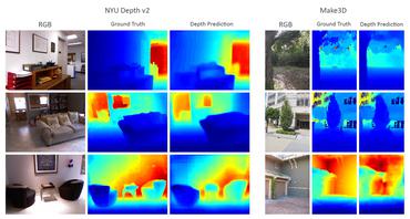
Introduction

Depth estimation is a crucial step towards inferring scene geometry from 2D images. The goal in monocular depth estimation is to predict the depth value of each pixel or inferring depth information, given only a single RGB image as input. This example will show an approach to build a depth estimation model with a convnet and simple loss functions.

depth

Setup

import os

os.environ["KERAS_BACKEND"] = "tensorflow"

import sys

import tensorflow as tf
import keras
from keras import layers
from keras import ops
import pandas as pd
import numpy as np
import cv2
import matplotlib.pyplot as plt

keras.utils.set_random_seed(123)

Downloading the dataset

We will be using the dataset DIODE: A Dense Indoor and Outdoor Depth Dataset for this tutorial. However, we use the validation set generating training and evaluation subsets for our model. The reason we use the validation set rather than the training set of the original dataset is because the training set consists of 81GB of data, which is challenging to download compared to the validation set which is only 2.6GB. Other datasets that you could use are NYU-v2 and KITTI.

annotation_folder = "/dataset/"
if not os.path.exists(os.path.abspath(".") + annotation_folder):
    annotation_zip = keras.utils.get_file(
        "val.tar.gz",
        cache_subdir=os.path.abspath("."),
        origin="http://diode-dataset.s3.amazonaws.com/val.tar.gz",
        extract=True,
    )

Downloading data from http://diode-dataset.s3.amazonaws.com/val.tar.gz

2774625282/2774625282 ━━━━━━━━━━━━━━━━━━━━ 205s 0us/step

Preparing the dataset

We only use the indoor images to train our depth estimation model.

path = "val/indoors"

filelist = []

for root, dirs, files in os.walk(path):
    for file in files:
        filelist.append(os.path.join(root, file))

filelist.sort()
data = {
    "image": [x for x in filelist if x.endswith(".png")],
    "depth": [x for x in filelist if x.endswith("_depth.npy")],
    "mask": [x for x in filelist if x.endswith("_depth_mask.npy")],
}
df = pd.DataFrame(data)

df = df.sample(frac=1, random_state=42)

Preparing hyperparameters

HEIGHT = 256
WIDTH = 256
LR = 0.00001
EPOCHS = 30
BATCH_SIZE = 32

Building a data pipeline

The pipeline takes a dataframe containing the path for the RGB images, as well as the depth and depth mask files.
It reads and resize the RGB images.
It reads the depth and depth mask files, process them to generate the depth map image and resize it.
It returns the RGB images and the depth map images for a batch.

class DataGenerator(keras.utils.PyDataset):
    def __init__(self, data, batch_size=6, dim=(768, 1024), n_channels=3, shuffle=True):
        super().__init__()
        """
        Initialization
        """
        self.data = data
        self.indices = self.data.index.tolist()
        self.dim = dim
        self.n_channels = n_channels
        self.batch_size = batch_size
        self.shuffle = shuffle
        self.min_depth = 0.1
        self.on_epoch_end()

    def __len__(self):
        return int(np.ceil(len(self.data) / self.batch_size))

    def __getitem__(self, index):
        if (index + 1) * self.batch_size > len(self.indices):
            self.batch_size = len(self.indices) - index * self.batch_size
        # Generate one batch of data
        # Generate indices of the batch
        index = self.indices[index * self.batch_size : (index + 1) * self.batch_size]
        # Find list of IDs
        batch = [self.indices[k] for k in index]
        x, y = self.data_generation(batch)

        return x, y

    def on_epoch_end(self):
        """
        Updates indexes after each epoch
        """
        self.index = np.arange(len(self.indices))
        if self.shuffle == True:
            np.random.shuffle(self.index)

    def load(self, image_path, depth_map, mask):
        """Load input and target image."""

        image_ = cv2.imread(image_path)
        image_ = cv2.cvtColor(image_, cv2.COLOR_BGR2RGB)
        image_ = cv2.resize(image_, self.dim)
        image_ = tf.image.convert_image_dtype(image_, tf.float32)

        depth_map = np.load(depth_map).squeeze()

        mask = np.load(mask)
        mask = mask > 0

        max_depth = min(300, np.percentile(depth_map, 99))
        depth_map = np.clip(depth_map, self.min_depth, max_depth)
        depth_map = np.log(depth_map, where=mask)

        depth_map = np.ma.masked_where(~mask, depth_map)

        depth_map = np.clip(depth_map, 0.1, np.log(max_depth))
        depth_map = cv2.resize(depth_map, self.dim)
        depth_map = np.expand_dims(depth_map, axis=2)
        depth_map = tf.image.convert_image_dtype(depth_map, tf.float32)

        return image_, depth_map

    def data_generation(self, batch):
        x = np.empty((self.batch_size, *self.dim, self.n_channels))
        y = np.empty((self.batch_size, *self.dim, 1))

        for i, batch_id in enumerate(batch):
            x[i,], y[i,] = self.load(
                self.data["image"][batch_id],
                self.data["depth"][batch_id],
                self.data["mask"][batch_id],
            )
        x, y = x.astype("float32"), y.astype("float32")
        return x, y

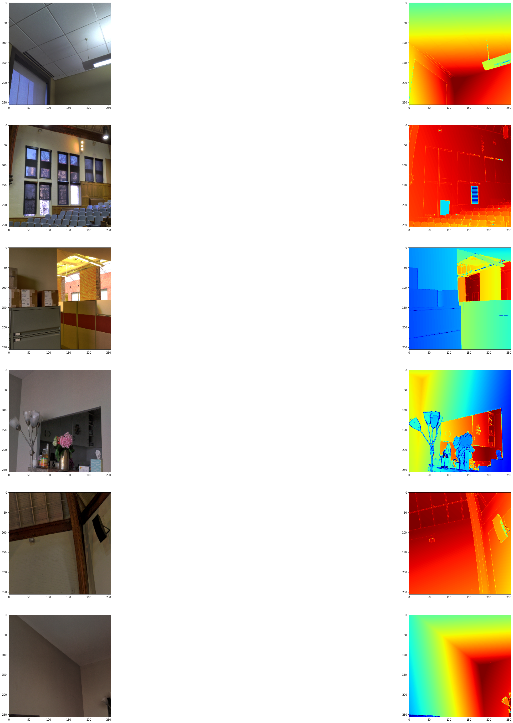
Visualizing samples

def visualize_depth_map(samples, test=False, model=None):
    input, target = samples
    cmap = plt.cm.jet
    cmap.set_bad(color="black")

    if test:
        pred = model.predict(input)
        fig, ax = plt.subplots(6, 3, figsize=(50, 50))
        for i in range(6):
            ax[i, 0].imshow((input[i].squeeze()))
            ax[i, 1].imshow((target[i].squeeze()), cmap=cmap)
            ax[i, 2].imshow((pred[i].squeeze()), cmap=cmap)

    else:
        fig, ax = plt.subplots(6, 2, figsize=(50, 50))
        for i in range(6):
            ax[i, 0].imshow((input[i].squeeze()))
            ax[i, 1].imshow((target[i].squeeze()), cmap=cmap)


visualize_samples = next(
    iter(DataGenerator(data=df, batch_size=6, dim=(HEIGHT, WIDTH)))
)
visualize_depth_map(visualize_samples)

png

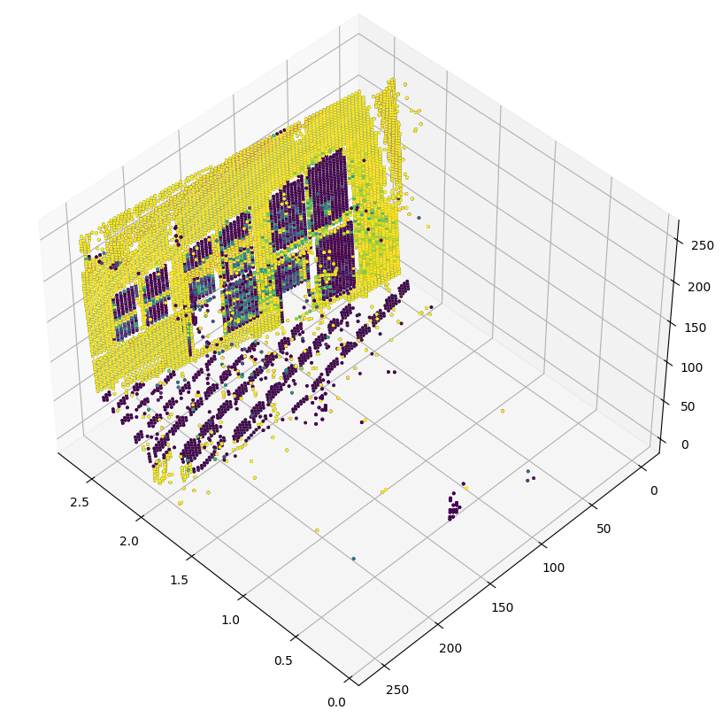
3D point cloud visualization

depth_vis = np.flipud(visualize_samples[1][1].squeeze())  # target
img_vis = np.flipud(visualize_samples[0][1].squeeze())  # input

fig = plt.figure(figsize=(15, 10))
ax = plt.axes(projection="3d")

STEP = 3
for x in range(0, img_vis.shape[0], STEP):
    for y in range(0, img_vis.shape[1], STEP):
        ax.scatter(
            [depth_vis[x, y]] * 3,
            [y] * 3,
            [x] * 3,
            c=tuple(img_vis[x, y, :3] / 255),
            s=3,
        )
    ax.view_init(45, 135)

png

Building the model

The basic model is from U-Net.
Addditive skip-connections are implemented in the downscaling block.

class DownscaleBlock(layers.Layer):
    def __init__(
        self, filters, kernel_size=(3, 3), padding="same", strides=1, **kwargs
    ):
        super().__init__(**kwargs)
        self.convA = layers.Conv2D(filters, kernel_size, strides, padding)
        self.convB = layers.Conv2D(filters, kernel_size, strides, padding)
        self.reluA = layers.LeakyReLU(negative_slope=0.2)
        self.reluB = layers.LeakyReLU(negative_slope=0.2)
        self.bn2a = layers.BatchNormalization()
        self.bn2b = layers.BatchNormalization()

        self.pool = layers.MaxPool2D((2, 2), (2, 2))

    def call(self, input_tensor):
        d = self.convA(input_tensor)
        x = self.bn2a(d)
        x = self.reluA(x)

        x = self.convB(x)
        x = self.bn2b(x)
        x = self.reluB(x)

        x += d
        p = self.pool(x)
        return x, p


class UpscaleBlock(layers.Layer):
    def __init__(
        self, filters, kernel_size=(3, 3), padding="same", strides=1, **kwargs
    ):
        super().__init__(**kwargs)
        self.us = layers.UpSampling2D((2, 2))
        self.convA = layers.Conv2D(filters, kernel_size, strides, padding)
        self.convB = layers.Conv2D(filters, kernel_size, strides, padding)
        self.reluA = layers.LeakyReLU(negative_slope=0.2)
        self.reluB = layers.LeakyReLU(negative_slope=0.2)
        self.bn2a = layers.BatchNormalization()
        self.bn2b = layers.BatchNormalization()
        self.conc = layers.Concatenate()

    def call(self, x, skip):
        x = self.us(x)
        concat = self.conc([x, skip])
        x = self.convA(concat)
        x = self.bn2a(x)
        x = self.reluA(x)

        x = self.convB(x)
        x = self.bn2b(x)
        x = self.reluB(x)

        return x


class BottleNeckBlock(layers.Layer):
    def __init__(
        self, filters, kernel_size=(3, 3), padding="same", strides=1, **kwargs
    ):
        super().__init__(**kwargs)
        self.convA = layers.Conv2D(filters, kernel_size, strides, padding)
        self.convB = layers.Conv2D(filters, kernel_size, strides, padding)
        self.reluA = layers.LeakyReLU(negative_slope=0.2)
        self.reluB = layers.LeakyReLU(negative_slope=0.2)

    def call(self, x):
        x = self.convA(x)
        x = self.reluA(x)
        x = self.convB(x)
        x = self.reluB(x)
        return x

Defining the loss

We will optimize 3 losses in our mode. 1. Structural similarity index(SSIM). 2. L1-loss, or Point-wise depth in our case. 3. Depth smoothness loss.

Out of the three loss functions, SSIM contributes the most to improving model performance.

def image_gradients(image):
    if len(ops.shape(image)) != 4:
        raise ValueError(
            "image_gradients expects a 4D tensor "
            "[batch_size, h, w, d], not {}.".format(ops.shape(image))
        )

    image_shape = ops.shape(image)
    batch_size, height, width, depth = ops.unstack(image_shape)

    dy = image[:, 1:, :, :] - image[:, :-1, :, :]
    dx = image[:, :, 1:, :] - image[:, :, :-1, :]

    # Return tensors with same size as original image by concatenating
    # zeros. Place the gradient [I(x+1,y) - I(x,y)] on the base pixel (x, y).
    shape = ops.stack([batch_size, 1, width, depth])
    dy = ops.concatenate([dy, ops.zeros(shape, dtype=image.dtype)], axis=1)
    dy = ops.reshape(dy, image_shape)

    shape = ops.stack([batch_size, height, 1, depth])
    dx = ops.concatenate([dx, ops.zeros(shape, dtype=image.dtype)], axis=2)
    dx = ops.reshape(dx, image_shape)

    return dy, dx


class DepthEstimationModel(keras.Model):
    def __init__(self):
        super().__init__()
        self.ssim_loss_weight = 0.85
        self.l1_loss_weight = 0.1
        self.edge_loss_weight = 0.9
        self.loss_metric = keras.metrics.Mean(name="loss")
        f = [16, 32, 64, 128, 256]
        self.downscale_blocks = [
            DownscaleBlock(f[0]),
            DownscaleBlock(f[1]),
            DownscaleBlock(f[2]),
            DownscaleBlock(f[3]),
        ]
        self.bottle_neck_block = BottleNeckBlock(f[4])
        self.upscale_blocks = [
            UpscaleBlock(f[3]),
            UpscaleBlock(f[2]),
            UpscaleBlock(f[1]),
            UpscaleBlock(f[0]),
        ]
        self.conv_layer = layers.Conv2D(1, (1, 1), padding="same", activation="tanh")

    def calculate_loss(self, target, pred):
        # Edges
        dy_true, dx_true = image_gradients(target)
        dy_pred, dx_pred = image_gradients(pred)
        weights_x = ops.cast(ops.exp(ops.mean(ops.abs(dx_true))), "float32")
        weights_y = ops.cast(ops.exp(ops.mean(ops.abs(dy_true))), "float32")

        # Depth smoothness
        smoothness_x = dx_pred * weights_x
        smoothness_y = dy_pred * weights_y

        depth_smoothness_loss = ops.mean(abs(smoothness_x)) + ops.mean(
            abs(smoothness_y)
        )

        # Structural similarity (SSIM) index
        ssim_loss = ops.mean(
            1
            - tf.image.ssim(
                target, pred, max_val=WIDTH, filter_size=7, k1=0.01**2, k2=0.03**2
            )
        )
        # Point-wise depth
        l1_loss = ops.mean(ops.abs(target - pred))

        loss = (
            (self.ssim_loss_weight * ssim_loss)
            + (self.l1_loss_weight * l1_loss)
            + (self.edge_loss_weight * depth_smoothness_loss)
        )

        return loss

    @property
    def metrics(self):
        return [self.loss_metric]

    def train_step(self, batch_data):
        input, target = batch_data
        with tf.GradientTape() as tape:
            pred = self(input, training=True)
            loss = self.calculate_loss(target, pred)

        gradients = tape.gradient(loss, self.trainable_variables)
        self.optimizer.apply_gradients(zip(gradients, self.trainable_variables))
        self.loss_metric.update_state(loss)
        return {
            "loss": self.loss_metric.result(),
        }

    def test_step(self, batch_data):
        input, target = batch_data

        pred = self(input, training=False)
        loss = self.calculate_loss(target, pred)

        self.loss_metric.update_state(loss)
        return {
            "loss": self.loss_metric.result(),
        }

    def call(self, x):
        c1, p1 = self.downscale_blocks[0](x)
        c2, p2 = self.downscale_blocks[1](p1)
        c3, p3 = self.downscale_blocks[2](p2)
        c4, p4 = self.downscale_blocks[3](p3)

        bn = self.bottle_neck_block(p4)

        u1 = self.upscale_blocks[0](bn, c4)
        u2 = self.upscale_blocks[1](u1, c3)
        u3 = self.upscale_blocks[2](u2, c2)
        u4 = self.upscale_blocks[3](u3, c1)

        return self.conv_layer(u4)

Model training

optimizer = keras.optimizers.SGD(
    learning_rate=LR,
    nesterov=False,
)
model = DepthEstimationModel()
# Compile the model
model.compile(optimizer)

train_loader = DataGenerator(
    data=df[:260].reset_index(drop="true"), batch_size=BATCH_SIZE, dim=(HEIGHT, WIDTH)
)
validation_loader = DataGenerator(
    data=df[260:].reset_index(drop="true"), batch_size=BATCH_SIZE, dim=(HEIGHT, WIDTH)
)
model.fit(
    train_loader,
    epochs=EPOCHS,
    validation_data=validation_loader,
)

Epoch 1/30
 9/9 ━━━━━━━━━━━━━━━━━━━━ 64s 5s/step - loss: 0.7656 - val_loss: 0.7738
Epoch 10/30
 9/9 ━━━━━━━━━━━━━━━━━━━━ 7s 602ms/step - loss: 0.7005 - val_loss: 0.6696
Epoch 20/30
 9/9 ━━━━━━━━━━━━━━━━━━━━ 7s 632ms/step - loss: 0.5827 - val_loss: 0.5821
Epoch 30/30
 9/9 ━━━━━━━━━━━━━━━━━━━━ 7s 593ms/step - loss: 0.6218 - val_loss: 0.5132

<keras.src.callbacks.history.History at 0x7f5a2886d210>

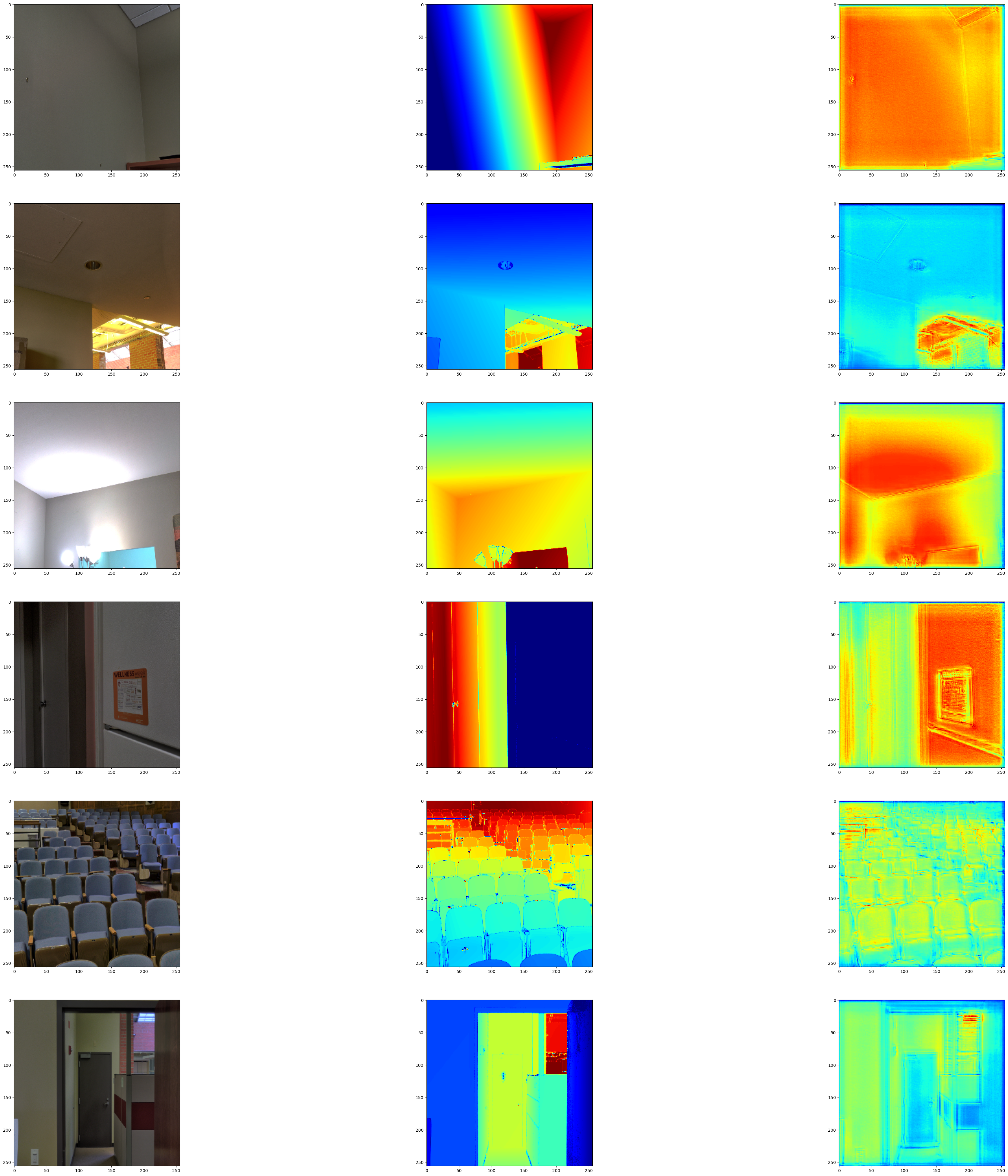
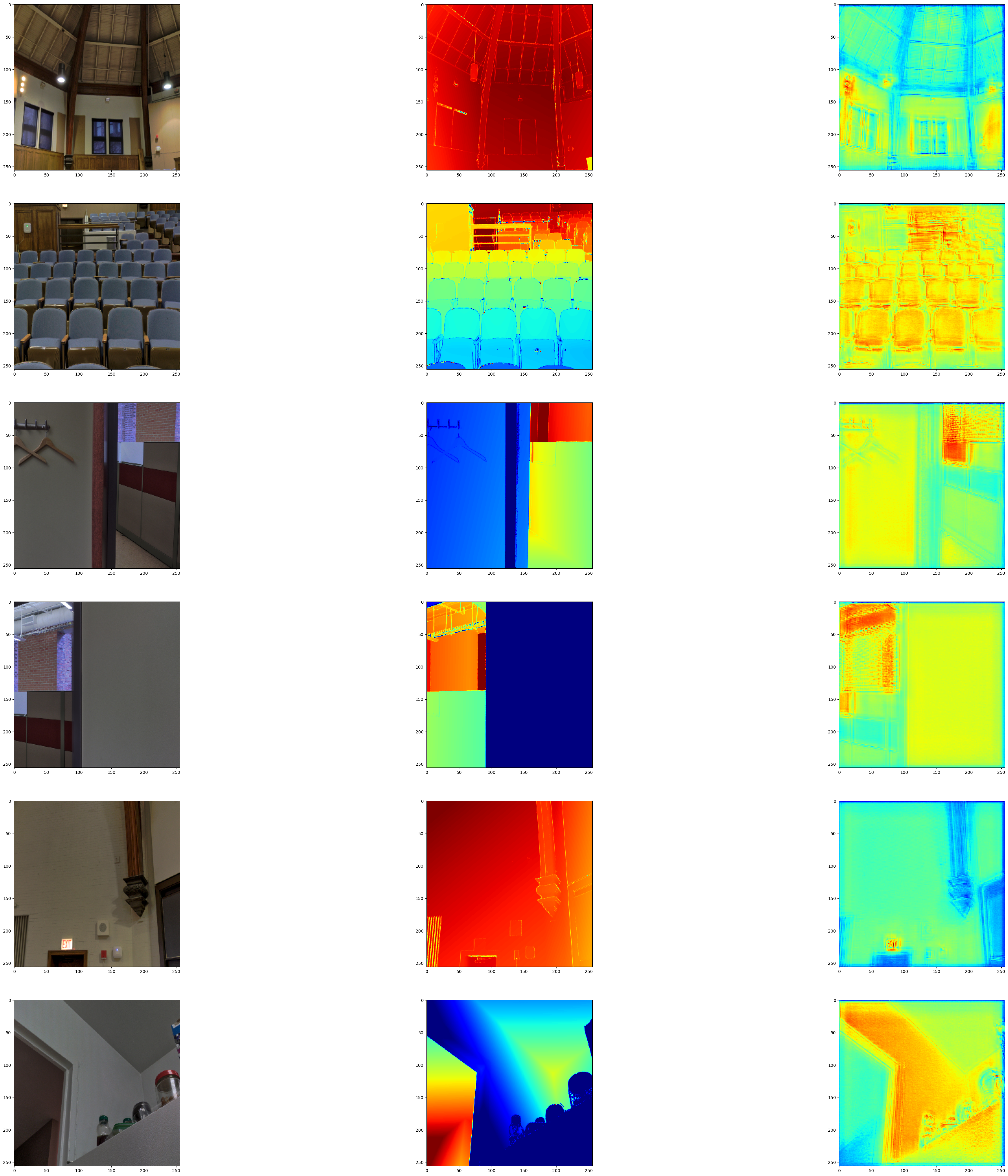
Visualizing model output

We visualize the model output over the validation set. The first image is the RGB image, the second image is the ground truth depth map image and the third one is the predicted depth map image.

test_loader = next(
    iter(
        DataGenerator(
            data=df[265:].reset_index(drop="true"), batch_size=6, dim=(HEIGHT, WIDTH)
        )
    )
)
visualize_depth_map(test_loader, test=True, model=model)

test_loader = next(
    iter(
        DataGenerator(
            data=df[300:].reset_index(drop="true"), batch_size=6, dim=(HEIGHT, WIDTH)
        )
    )
)
visualize_depth_map(test_loader, test=True, model=model)

1/1 ━━━━━━━━━━━━━━━━━━━━ 0s 781ms/step

1/1 ━━━━━━━━━━━━━━━━━━━━ 1s 782ms/step

1/1 ━━━━━━━━━━━━━━━━━━━━ 0s 171ms/step

1/1 ━━━━━━━━━━━━━━━━━━━━ 0s 172ms/step

png

Possible improvements

You can improve this model by replacing the encoding part of the U-Net with a pretrained DenseNet or ResNet.
Loss functions play an important role in solving this problem. Tuning the loss functions may yield significant improvement.