Consistency training with supervision
Author: Sayak Paul
Date created: 2021/04/13
Last modified: 2021/04/19
Description: Training with consistency regularization for robustness against data distribution shifts.

Deep learning models excel in many image recognition tasks when the data is independent and identically distributed (i.i.d.). However, they can suffer from performance degradation caused by subtle distribution shifts in the input data (such as random noise, contrast change, and blurring). So, naturally, there arises a question of why. As discussed in A Fourier Perspective on Model Robustness in Computer Vision), there's no reason for deep learning models to be robust against such shifts. Standard model training procedures (such as standard image classification training workflows) don't enable a model to learn beyond what's fed to it in the form of training data.
In this example, we will be training an image classification model enforcing a sense of consistency inside it by doing the following:
- Train a standard image classification model.
- Train an equal or larger model on a noisy version of the dataset (augmented using RandAugment).
- To do this, we will first obtain predictions of the previous model on the clean images of the dataset.
- We will then use these predictions and train the second model to match these predictions on the noisy variant of the same images. This is identical to the workflow of Knowledge Distillation but since the student model is equal or larger in size this process is also referred to as Self-Training.
This overall training workflow finds its roots in works like FixMatch, Unsupervised Data Augmentation for Consistency Training, and Noisy Student Training. Since this training process encourages a model yield consistent predictions for clean as well as noisy images, it's often referred to as consistency training or training with consistency regularization. Although the example focuses on using consistency training to enhance the robustness of models to common corruptions this example can also serve a template for performing weakly supervised learning.
This example requires TensorFlow 2.4 or higher, as well as TensorFlow Hub and TensorFlow Models, which can be installed using the following command:
!pip install -q tf-models-official tensorflow-addons
Imports and setup
from official.vision.image_classification.augment import RandAugment
from tensorflow.keras import layers

import tensorflow as tf
import tensorflow_addons as tfa
import matplotlib.pyplot as plt

tf.random.set_seed(42)
Define hyperparameters
AUTO = tf.data.AUTOTUNE
BATCH_SIZE = 128
EPOCHS = 5

CROP_TO = 72
RESIZE_TO = 96
Load the CIFAR-10 dataset
(x_train, y_train), (x_test, y_test) = tf.keras.datasets.cifar10.load_data()

val_samples = 49500
new_train_x, new_y_train = x_train[: val_samples + 1], y_train[: val_samples + 1]
val_x, val_y = x_train[val_samples:], y_train[val_samples:]
Create TensorFlow Dataset objects
# Initialize `RandAugment` object with 2 layers of
# augmentation transforms and strength of 9.
augmenter = RandAugment(num_layers=2, magnitude=9)
For training the teacher model, we will only be using two geometric augmentation transforms: random horizontal flip and random crop.
def preprocess_train(image, label, noisy=True):
    image = tf.image.random_flip_left_right(image)
    # We first resize the original image to a larger dimension
    # and then we take random crops from it.
    image = tf.image.resize(image, [RESIZE_TO, RESIZE_TO])
    image = tf.image.random_crop(image, [CROP_TO, CROP_TO, 3])
    if noisy:
        image = augmenter.distort(image)
    return image, label


def preprocess_test(image, label):
    image = tf.image.resize(image, [CROP_TO, CROP_TO])
    return image, label


train_ds = tf.data.Dataset.from_tensor_slices((new_train_x, new_y_train))
validation_ds = tf.data.Dataset.from_tensor_slices((val_x, val_y))
test_ds = tf.data.Dataset.from_tensor_slices((x_test, y_test))
We make sure train_clean_ds and train_noisy_ds are shuffled using the same seed to
ensure their orders are exactly the same. This will be helpful during training the
student model.
# This dataset will be used to train the first model.
train_clean_ds = (
    train_ds.shuffle(BATCH_SIZE * 10, seed=42)
    .map(lambda x, y: (preprocess_train(x, y, noisy=False)), num_parallel_calls=AUTO)
    .batch(BATCH_SIZE)
    .prefetch(AUTO)
)

# This prepares the `Dataset` object to use RandAugment.
train_noisy_ds = (
    train_ds.shuffle(BATCH_SIZE * 10, seed=42)
    .map(preprocess_train, num_parallel_calls=AUTO)
    .batch(BATCH_SIZE)
    .prefetch(AUTO)
)

validation_ds = (
    validation_ds.map(preprocess_test, num_parallel_calls=AUTO)
    .batch(BATCH_SIZE)
    .prefetch(AUTO)
)

test_ds = (
    test_ds.map(preprocess_test, num_parallel_calls=AUTO)
    .batch(BATCH_SIZE)
    .prefetch(AUTO)
)

# This dataset will be used to train the second model.
consistency_training_ds = tf.data.Dataset.zip((train_clean_ds, train_noisy_ds))
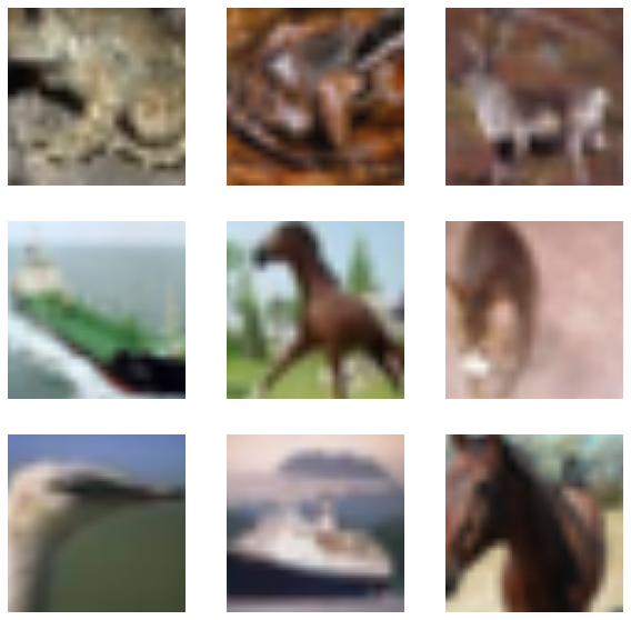
Visualize the datasets
sample_images, sample_labels = next(iter(train_clean_ds))
plt.figure(figsize=(10, 10))
for i, image in enumerate(sample_images[:9]):
ax = plt.subplot(3, 3, i + 1)
plt.imshow(image.numpy().astype("int"))
plt.axis("off")
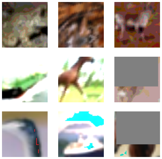
sample_images, sample_labels = next(iter(train_noisy_ds))
plt.figure(figsize=(10, 10))
for i, image in enumerate(sample_images[:9]):
ax = plt.subplot(3, 3, i + 1)
plt.imshow(image.numpy().astype("int"))
plt.axis("off")
Define a model building utility function
We now define our model building utility. Our model is based on the ResNet50V2 architecture.
def get_training_model(num_classes=10):
    resnet50_v2 = tf.keras.applications.ResNet50V2(
        weights=None, include_top=False, input_shape=(CROP_TO, CROP_TO, 3),
    )
    model = tf.keras.Sequential(
        [
            layers.Input((CROP_TO, CROP_TO, 3)),
            layers.Rescaling(scale=1.0 / 127.5, offset=-1),
            resnet50_v2,
            layers.GlobalAveragePooling2D(),
            layers.Dense(num_classes),
        ]
    )
    return model
In the interest of reproducibility, we serialize the initial random weights of the teacher network.
initial_teacher_model = get_training_model()
initial_teacher_model.save_weights("initial_teacher_model.h5")
Train the teacher model
As noted in Noisy Student Training, if the teacher model is trained with geometric ensembling and when the student model is forced to mimic that, it leads to better performance. The original work uses Stochastic Depth and Dropout to bring in the ensembling part but for this example, we will use Stochastic Weight Averaging (SWA) which also resembles geometric ensembling.
# Define the callbacks.
reduce_lr = tf.keras.callbacks.ReduceLROnPlateau(patience=3)
early_stopping = tf.keras.callbacks.EarlyStopping(
    patience=10, restore_best_weights=True
)

# Initialize SWA from tf-hub.
SWA = tfa.optimizers.SWA

# Compile and train the teacher model.
teacher_model = get_training_model()
teacher_model.load_weights("initial_teacher_model.h5")
teacher_model.compile(
    # Notice that we are wrapping our optimizer within SWA
    optimizer=SWA(tf.keras.optimizers.Adam()),
    loss=tf.keras.losses.SparseCategoricalCrossentropy(from_logits=True),
    metrics=["accuracy"],
)
history = teacher_model.fit(
    train_clean_ds,
    epochs=EPOCHS,
    validation_data=validation_ds,
    callbacks=[reduce_lr, early_stopping],
)

# Evaluate the teacher model on the test set.
_, acc = teacher_model.evaluate(test_ds, verbose=0)
print(f"Test accuracy: {acc*100}%")
Epoch 1/5
387/387 [==============================] - 73s 78ms/step - loss: 1.7785 - accuracy: 0.3582 - val_loss: 2.0589 - val_accuracy: 0.3920
Epoch 2/5
387/387 [==============================] - 28s 71ms/step - loss: 1.2493 - accuracy: 0.5542 - val_loss: 1.4228 - val_accuracy: 0.5380
Epoch 3/5
387/387 [==============================] - 28s 73ms/step - loss: 1.0294 - accuracy: 0.6350 - val_loss: 1.4422 - val_accuracy: 0.5900
Epoch 4/5
387/387 [==============================] - 28s 73ms/step - loss: 0.8954 - accuracy: 0.6864 - val_loss: 1.2189 - val_accuracy: 0.6520
Epoch 5/5
387/387 [==============================] - 28s 73ms/step - loss: 0.7879 - accuracy: 0.7231 - val_loss: 0.9790 - val_accuracy: 0.6500
Test accuracy: 65.83999991416931%
Define a self-training utility
For this part, we will borrow the Distiller class from this Keras Example.
# Majority of the code is taken from:
# https://keras.io/examples/vision/knowledge_distillation/
class SelfTrainer(tf.keras.Model):
    def __init__(self, student, teacher):
        super().__init__()
        self.student = student
        self.teacher = teacher

    def compile(
        self, optimizer, metrics, student_loss_fn, distillation_loss_fn, temperature=3,
    ):
        super().compile(optimizer=optimizer, metrics=metrics)
        self.student_loss_fn = student_loss_fn
        self.distillation_loss_fn = distillation_loss_fn
        self.temperature = temperature

    def train_step(self, data):
        # Since our dataset is a zip of two independent datasets,
        # after initially parsing them, we segregate the
        # respective images and labels next.
        clean_ds, noisy_ds = data
        clean_images, _ = clean_ds
        noisy_images, y = noisy_ds

        # Forward pass of teacher
        teacher_predictions = self.teacher(clean_images, training=False)

        with tf.GradientTape() as tape:
            # Forward pass of student
            student_predictions = self.student(noisy_images, training=True)

            # Compute losses
            student_loss = self.student_loss_fn(y, student_predictions)
            distillation_loss = self.distillation_loss_fn(
                tf.nn.softmax(teacher_predictions / self.temperature, axis=1),
                tf.nn.softmax(student_predictions / self.temperature, axis=1),
            )
            total_loss = (student_loss + distillation_loss) / 2

        # Compute gradients
        trainable_vars = self.student.trainable_variables
        gradients = tape.gradient(total_loss, trainable_vars)

        # Update weights
        self.optimizer.apply_gradients(zip(gradients, trainable_vars))

        # Update the metrics configured in `compile()`
        self.compiled_metrics.update_state(
            y, tf.nn.softmax(student_predictions, axis=1)
        )

        # Return a dict of performance
        results = {m.name: m.result() for m in self.metrics}
        results.update({"total_loss": total_loss})
        return results

    def test_step(self, data):
        # During inference, we only pass a dataset consisting images and labels.
        x, y = data

        # Compute predictions
        y_prediction = self.student(x, training=False)

        # Update the metrics
        self.compiled_metrics.update_state(y, tf.nn.softmax(y_prediction, axis=1))

        # Return a dict of performance
        results = {m.name: m.result() for m in self.metrics}
        return results
The only difference in this implementation is the way loss is being calculated. Instead of weighted the distillation loss and student loss differently we are taking their average following Noisy Student Training.
Train the student model
# Define the callbacks.
# We are using a larger decay factor to stabilize the training.
reduce_lr = tf.keras.callbacks.ReduceLROnPlateau(
    patience=3, factor=0.5, monitor="val_accuracy"
)
early_stopping = tf.keras.callbacks.EarlyStopping(
    patience=10, restore_best_weights=True, monitor="val_accuracy"
)

# Compile and train the student model.
self_trainer = SelfTrainer(student=get_training_model(), teacher=teacher_model)
self_trainer.compile(
    # Notice we are *not* using SWA here.
    optimizer="adam",
    metrics=["accuracy"],
    student_loss_fn=tf.keras.losses.SparseCategoricalCrossentropy(from_logits=True),
    distillation_loss_fn=tf.keras.losses.KLDivergence(),
    temperature=10,
)
history = self_trainer.fit(
    consistency_training_ds,
    epochs=EPOCHS,
    validation_data=validation_ds,
    callbacks=[reduce_lr, early_stopping],
)

# Evaluate the student model.
acc = self_trainer.evaluate(test_ds, verbose=0)
print(f"Test accuracy from student model: {acc*100}%")
Epoch 1/5
387/387 [==============================] - 39s 84ms/step - accuracy: 0.2112 - total_loss: 1.0629 - val_accuracy: 0.4180
Epoch 2/5
387/387 [==============================] - 32s 82ms/step - accuracy: 0.3341 - total_loss: 0.9554 - val_accuracy: 0.3900
Epoch 3/5
387/387 [==============================] - 31s 81ms/step - accuracy: 0.3873 - total_loss: 0.8852 - val_accuracy: 0.4580
Epoch 4/5
387/387 [==============================] - 31s 81ms/step - accuracy: 0.4294 - total_loss: 0.8423 - val_accuracy: 0.5660
Epoch 5/5
387/387 [==============================] - 31s 81ms/step - accuracy: 0.4547 - total_loss: 0.8093 - val_accuracy: 0.5880
Test accuracy from student model: 58.490002155303955%
Assess the robustness of the models
A standard benchmark of assessing the robustness of vision models is to record their performance on corrupted datasets like ImageNet-C and CIFAR-10-C both of which were proposed in Benchmarking Neural Network Robustness to Common Corruptions and Perturbations. For this example, we will be using the CIFAR-10-C dataset which has 19 different corruptions on 5 different severity levels. To assess the robustness of the models on this dataset, we will do the following:
- Run the pre-trained models on the highest level of severities and obtain the top-1 accuracies.
- Compute the mean top-1 accuracy.
For the purpose of this example, we won't be going through these steps. This is why we trained the models for only 5 epochs. You can check out this repository that demonstrates the full-scale training experiments and also the aforementioned assessment. The figure below presents an executive summary of that assessment:

Mean Top-1 results stand for the CIFAR-10-C dataset and Test Top-1 results stand for the CIFAR-10 test set. It's clear that consistency training has an advantage on not only enhancing the model robustness but also on improving the standard test performance.