► Code examples / Timeseries / Traffic forecasting using graph neural networks and LSTM

Traffic forecasting using graph neural networks and LSTM

Author: Arash Khodadadi
Date created: 2021/12/28
Last modified: 2023/11/22
Description: This example demonstrates how to do timeseries forecasting over graphs.

ⓘ This example uses Keras 3

View in Colab • GitHub source

Introduction

This example shows how to forecast traffic condition using graph neural networks and LSTM. Specifically, we are interested in predicting the future values of the traffic speed given a history of the traffic speed for a collection of road segments.

One popular method to solve this problem is to consider each road segment's traffic speed as a separate timeseries and predict the future values of each timeseries using the past values of the same timeseries.

This method, however, ignores the dependency of the traffic speed of one road segment on the neighboring segments. To be able to take into account the complex interactions between the traffic speed on a collection of neighboring roads, we can define the traffic network as a graph and consider the traffic speed as a signal on this graph. In this example, we implement a neural network architecture which can process timeseries data over a graph. We first show how to process the data and create a tf.data.Dataset for forecasting over graphs. Then, we implement a model which uses graph convolution and LSTM layers to perform forecasting over a graph.

The data processing and the model architecture are inspired by this paper:

Yu, Bing, Haoteng Yin, and Zhanxing Zhu. "Spatio-temporal graph convolutional networks: a deep learning framework for traffic forecasting." Proceedings of the 27th International Joint Conference on Artificial Intelligence, 2018. (github)

Setup

import os

os.environ["KERAS_BACKEND"] = "tensorflow"

import pandas as pd
import numpy as np
import typing
import matplotlib.pyplot as plt

import tensorflow as tf
import keras
from keras import layers
from keras import ops

Data preparation

Data description

We use a real-world traffic speed dataset named PeMSD7. We use the version collected and prepared by Yu et al., 2018 and available here.

The data consists of two files:

PeMSD7_W_228.csv contains the distances between 228 stations across the District 7 of California.
PeMSD7_V_228.csv contains traffic speed collected for those stations in the weekdays of May and June of 2012.

The full description of the dataset can be found in Yu et al., 2018.

Loading data

url = "https://github.com/VeritasYin/STGCN_IJCAI-18/raw/master/dataset/PeMSD7_Full.zip"
data_dir = keras.utils.get_file(origin=url, extract=True, archive_format="zip")
data_dir = data_dir.rstrip("PeMSD7_Full.zip")

route_distances = pd.read_csv(
    os.path.join(data_dir, "PeMSD7_W_228.csv"), header=None
).to_numpy()
speeds_array = pd.read_csv(
    os.path.join(data_dir, "PeMSD7_V_228.csv"), header=None
).to_numpy()

print(f"route_distances shape={route_distances.shape}")
print(f"speeds_array shape={speeds_array.shape}")

route_distances shape=(228, 228)
speeds_array shape=(12672, 228)

sub-sampling roads

To reduce the problem size and make the training faster, we will only work with a sample of 26 roads out of the 228 roads in the dataset. We have chosen the roads by starting from road 0, choosing the 5 closest roads to it, and continuing this process until we get 25 roads. You can choose any other subset of the roads. We chose the roads in this way to increase the likelihood of having roads with correlated speed timeseries. sample_routes contains the IDs of the selected roads.

sample_routes = [
    0,
    1,
    4,
    7,
    8,
    11,
    15,
    108,
    109,
    114,
    115,
    118,
    120,
    123,
    124,
    126,
    127,
    129,
    130,
    132,
    133,
    136,
    139,
    144,
    147,
    216,
]
route_distances = route_distances[np.ix_(sample_routes, sample_routes)]
speeds_array = speeds_array[:, sample_routes]

print(f"route_distances shape={route_distances.shape}")
print(f"speeds_array shape={speeds_array.shape}")

route_distances shape=(26, 26)
speeds_array shape=(12672, 26)

Data visualization

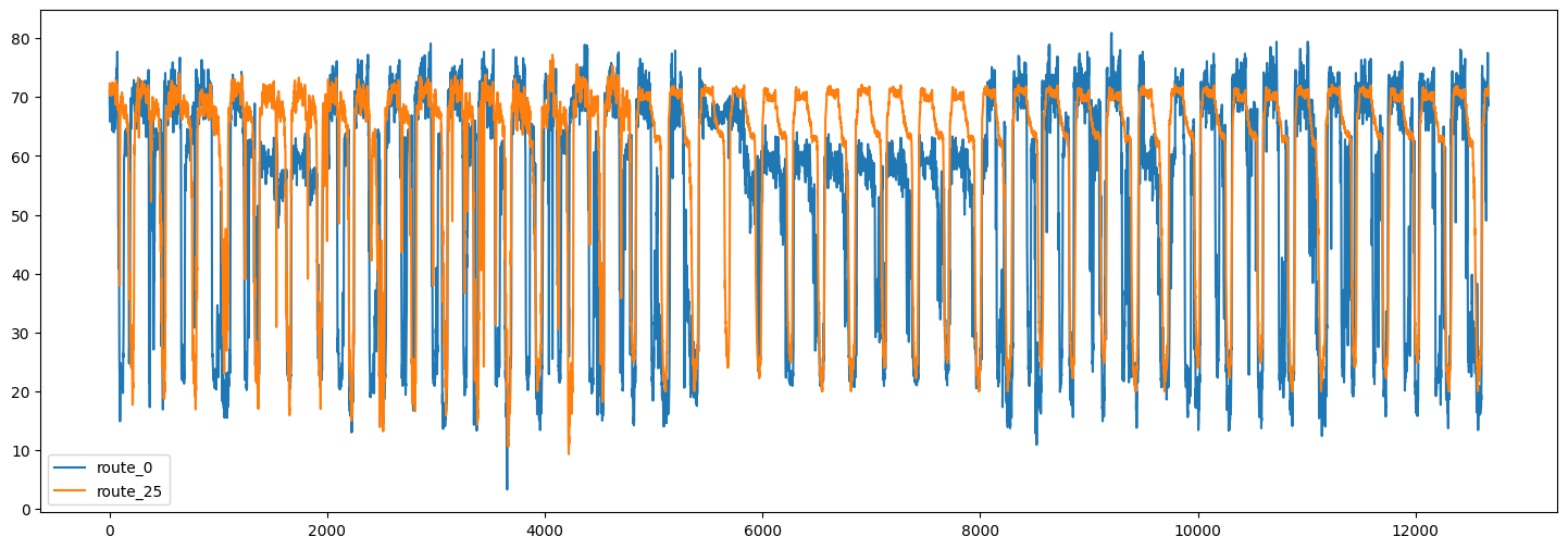
Here are the timeseries of the traffic speed for two of the routes:

plt.figure(figsize=(18, 6))
plt.plot(speeds_array[:, [0, -1]])
plt.legend(["route_0", "route_25"])

<matplotlib.legend.Legend at 0x7f5a870b2050>

png

We can also visualize the correlation between the timeseries in different routes.

plt.figure(figsize=(8, 8))
plt.matshow(np.corrcoef(speeds_array.T), 0)
plt.xlabel("road number")
plt.ylabel("road number")

Text(0, 0.5, 'road number')

png

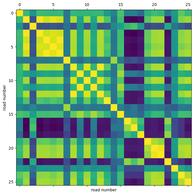
Using this correlation heatmap, we can see that for example the speed in routes 4, 5, 6 are highly correlated.

Splitting and normalizing data

Next, we split the speed values array into train/validation/test sets, and normalize the resulting arrays:

train_size, val_size = 0.5, 0.2


def preprocess(data_array: np.ndarray, train_size: float, val_size: float):
    """Splits data into train/val/test sets and normalizes the data.

    Args:
        data_array: ndarray of shape `(num_time_steps, num_routes)`
        train_size: A float value between 0.0 and 1.0 that represent the proportion of the dataset
            to include in the train split.
        val_size: A float value between 0.0 and 1.0 that represent the proportion of the dataset
            to include in the validation split.

    Returns:
        `train_array`, `val_array`, `test_array`
    """

    num_time_steps = data_array.shape[0]
    num_train, num_val = (
        int(num_time_steps * train_size),
        int(num_time_steps * val_size),
    )
    train_array = data_array[:num_train]
    mean, std = train_array.mean(axis=0), train_array.std(axis=0)

    train_array = (train_array - mean) / std
    val_array = (data_array[num_train : (num_train + num_val)] - mean) / std
    test_array = (data_array[(num_train + num_val) :] - mean) / std

    return train_array, val_array, test_array


train_array, val_array, test_array = preprocess(speeds_array, train_size, val_size)

print(f"train set size: {train_array.shape}")
print(f"validation set size: {val_array.shape}")
print(f"test set size: {test_array.shape}")

train set size: (6336, 26)
validation set size: (2534, 26)
test set size: (3802, 26)

Creating TensorFlow Datasets

Next, we create the datasets for our forecasting problem. The forecasting problem can be stated as follows: given a sequence of the road speed values at times t+1, t+2, ..., t+T, we want to predict the future values of the roads speed for times t+T+1, ..., t+T+h. So for each time t the inputs to our model are T vectors each of size N and the targets are h vectors each of size N, where N is the number of roads.

We use the Keras built-in function keras.utils.timeseries_dataset_from_array. The function create_tf_dataset() below takes as input a numpy.ndarray and returns a tf.data.Dataset. In this function input_sequence_length=T and forecast_horizon=h.

The argument multi_horizon needs more explanation. Assume forecast_horizon=3. If multi_horizon=True then the model will make a forecast for time steps t+T+1, t+T+2, t+T+3. So the target will have shape (T,3). But if multi_horizon=False, the model will make a forecast only for time step t+T+3 and so the target will have shape (T, 1).

You may notice that the input tensor in each batch has shape (batch_size, input_sequence_length, num_routes, 1). The last dimension is added to make the model more general: at each time step, the input features for each raod may contain multiple timeseries. For instance, one might want to use temperature timeseries in addition to historical values of the speed as input features. In this example, however, the last dimension of the input is always 1.

We use the last 12 values of the speed in each road to forecast the speed for 3 time steps ahead:

batch_size = 64
input_sequence_length = 12
forecast_horizon = 3
multi_horizon = False


def create_tf_dataset(
    data_array: np.ndarray,
    input_sequence_length: int,
    forecast_horizon: int,
    batch_size: int = 128,
    shuffle=True,
    multi_horizon=True,
):
    """Creates tensorflow dataset from numpy array.

    This function creates a dataset where each element is a tuple `(inputs, targets)`.
    `inputs` is a Tensor
    of shape `(batch_size, input_sequence_length, num_routes, 1)` containing
    the `input_sequence_length` past values of the timeseries for each node.
    `targets` is a Tensor of shape `(batch_size, forecast_horizon, num_routes)`
    containing the `forecast_horizon`
    future values of the timeseries for each node.

    Args:
        data_array: np.ndarray with shape `(num_time_steps, num_routes)`
        input_sequence_length: Length of the input sequence (in number of timesteps).
        forecast_horizon: If `multi_horizon=True`, the target will be the values of the timeseries for 1 to
            `forecast_horizon` timesteps ahead. If `multi_horizon=False`, the target will be the value of the
            timeseries `forecast_horizon` steps ahead (only one value).
        batch_size: Number of timeseries samples in each batch.
        shuffle: Whether to shuffle output samples, or instead draw them in chronological order.
        multi_horizon: See `forecast_horizon`.

    Returns:
        A tf.data.Dataset instance.
    """

    inputs = keras.utils.timeseries_dataset_from_array(
        np.expand_dims(data_array[:-forecast_horizon], axis=-1),
        None,
        sequence_length=input_sequence_length,
        shuffle=False,
        batch_size=batch_size,
    )

    target_offset = (
        input_sequence_length
        if multi_horizon
        else input_sequence_length + forecast_horizon - 1
    )
    target_seq_length = forecast_horizon if multi_horizon else 1
    targets = keras.utils.timeseries_dataset_from_array(
        data_array[target_offset:],
        None,
        sequence_length=target_seq_length,
        shuffle=False,
        batch_size=batch_size,
    )

    dataset = tf.data.Dataset.zip((inputs, targets))
    if shuffle:
        dataset = dataset.shuffle(100)

    return dataset.prefetch(16).cache()


train_dataset, val_dataset = (
    create_tf_dataset(data_array, input_sequence_length, forecast_horizon, batch_size)
    for data_array in [train_array, val_array]
)

test_dataset = create_tf_dataset(
    test_array,
    input_sequence_length,
    forecast_horizon,
    batch_size=test_array.shape[0],
    shuffle=False,
    multi_horizon=multi_horizon,
)

Roads Graph

As mentioned before, we assume that the road segments form a graph. The PeMSD7 dataset has the road segments distance. The next step is to create the graph adjacency matrix from these distances. Following Yu et al., 2018 (equation 10) we assume there is an edge between two nodes in the graph if the distance between the corresponding roads is less than a threshold.

def compute_adjacency_matrix(
    route_distances: np.ndarray, sigma2: float, epsilon: float
):
    """Computes the adjacency matrix from distances matrix.

    It uses the formula in https://github.com/VeritasYin/STGCN_IJCAI-18#data-preprocessing to
    compute an adjacency matrix from the distance matrix.
    The implementation follows that paper.

    Args:
        route_distances: np.ndarray of shape `(num_routes, num_routes)`. Entry `i,j` of this array is the
            distance between roads `i,j`.
        sigma2: Determines the width of the Gaussian kernel applied to the square distances matrix.
        epsilon: A threshold specifying if there is an edge between two nodes. Specifically, `A[i,j]=1`
            if `np.exp(-w2[i,j] / sigma2) >= epsilon` and `A[i,j]=0` otherwise, where `A` is the adjacency
            matrix and `w2=route_distances * route_distances`

    Returns:
        A boolean graph adjacency matrix.
    """
    num_routes = route_distances.shape[0]
    route_distances = route_distances / 10000.0
    w2, w_mask = (
        route_distances * route_distances,
        np.ones([num_routes, num_routes]) - np.identity(num_routes),
    )
    return (np.exp(-w2 / sigma2) >= epsilon) * w_mask

The function compute_adjacency_matrix() returns a boolean adjacency matrix where 1 means there is an edge between two nodes. We use the following class to store the information about the graph.

class GraphInfo:
    def __init__(self, edges: typing.Tuple[list, list], num_nodes: int):
        self.edges = edges
        self.num_nodes = num_nodes


sigma2 = 0.1
epsilon = 0.5
adjacency_matrix = compute_adjacency_matrix(route_distances, sigma2, epsilon)
node_indices, neighbor_indices = np.where(adjacency_matrix == 1)
graph = GraphInfo(
    edges=(node_indices.tolist(), neighbor_indices.tolist()),
    num_nodes=adjacency_matrix.shape[0],
)
print(f"number of nodes: {graph.num_nodes}, number of edges: {len(graph.edges[0])}")

number of nodes: 26, number of edges: 150

Network architecture

Our model for forecasting over the graph consists of a graph convolution layer and a LSTM layer.

Graph convolution layer

Our implementation of the graph convolution layer resembles the implementation in this Keras example. Note that in that example input to the layer is a 2D tensor of shape (num_nodes,in_feat) but in our example the input to the layer is a 4D tensor of shape (num_nodes, batch_size, input_seq_length, in_feat). The graph convolution layer performs the following steps:

The nodes' representations are computed in self.compute_nodes_representation() by multiplying the input features by self.weight
The aggregated neighbors' messages are computed in self.compute_aggregated_messages() by first aggregating the neighbors' representations and then multiplying the results by self.weight
The final output of the layer is computed in self.update() by combining the nodes representations and the neighbors' aggregated messages

class GraphConv(layers.Layer):
    def __init__(
        self,
        in_feat,
        out_feat,
        graph_info: GraphInfo,
        aggregation_type="mean",
        combination_type="concat",
        activation: typing.Optional[str] = None,
        **kwargs,
    ):
        super().__init__(**kwargs)
        self.in_feat = in_feat
        self.out_feat = out_feat
        self.graph_info = graph_info
        self.aggregation_type = aggregation_type
        self.combination_type = combination_type
        self.weight = self.add_weight(
            initializer=keras.initializers.GlorotUniform(),
            shape=(in_feat, out_feat),
            dtype="float32",
            trainable=True,
        )
        self.activation = layers.Activation(activation)

    def aggregate(self, neighbour_representations):
        aggregation_func = {
            "sum": tf.math.unsorted_segment_sum,
            "mean": tf.math.unsorted_segment_mean,
            "max": tf.math.unsorted_segment_max,
        }.get(self.aggregation_type)

        if aggregation_func:
            return aggregation_func(
                neighbour_representations,
                self.graph_info.edges[0],
                num_segments=self.graph_info.num_nodes,
            )

        raise ValueError(f"Invalid aggregation type: {self.aggregation_type}")

    def compute_nodes_representation(self, features):
        """Computes each node's representation.

        The nodes' representations are obtained by multiplying the features tensor with
        `self.weight`. Note that
        `self.weight` has shape `(in_feat, out_feat)`.

        Args:
            features: Tensor of shape `(num_nodes, batch_size, input_seq_len, in_feat)`

        Returns:
            A tensor of shape `(num_nodes, batch_size, input_seq_len, out_feat)`
        """
        return ops.matmul(features, self.weight)

    def compute_aggregated_messages(self, features):
        neighbour_representations = tf.gather(features, self.graph_info.edges[1])
        aggregated_messages = self.aggregate(neighbour_representations)
        return ops.matmul(aggregated_messages, self.weight)

    def update(self, nodes_representation, aggregated_messages):
        if self.combination_type == "concat":
            h = ops.concatenate([nodes_representation, aggregated_messages], axis=-1)
        elif self.combination_type == "add":
            h = nodes_representation + aggregated_messages
        else:
            raise ValueError(f"Invalid combination type: {self.combination_type}.")
        return self.activation(h)

    def call(self, features):
        """Forward pass.

        Args:
            features: tensor of shape `(num_nodes, batch_size, input_seq_len, in_feat)`

        Returns:
            A tensor of shape `(num_nodes, batch_size, input_seq_len, out_feat)`
        """
        nodes_representation = self.compute_nodes_representation(features)
        aggregated_messages = self.compute_aggregated_messages(features)
        return self.update(nodes_representation, aggregated_messages)

LSTM plus graph convolution

By applying the graph convolution layer to the input tensor, we get another tensor containing the nodes' representations over time (another 4D tensor). For each time step, a node's representation is informed by the information from its neighbors.

To make good forecasts, however, we need not only information from the neighbors but also we need to process the information over time. To this end, we can pass each node's tensor through a recurrent layer. The LSTMGC layer below, first applies a graph convolution layer to the inputs and then passes the results through a LSTM layer.

class LSTMGC(layers.Layer):
    """Layer comprising a convolution layer followed by LSTM and dense layers."""

    def __init__(
        self,
        in_feat,
        out_feat,
        lstm_units: int,
        input_seq_len: int,
        output_seq_len: int,
        graph_info: GraphInfo,
        graph_conv_params: typing.Optional[dict] = None,
        **kwargs,
    ):
        super().__init__(**kwargs)

        # graph conv layer
        if graph_conv_params is None:
            graph_conv_params = {
                "aggregation_type": "mean",
                "combination_type": "concat",
                "activation": None,
            }
        self.graph_conv = GraphConv(in_feat, out_feat, graph_info, **graph_conv_params)

        self.lstm = layers.LSTM(lstm_units, activation="relu")
        self.dense = layers.Dense(output_seq_len)

        self.input_seq_len, self.output_seq_len = input_seq_len, output_seq_len

    def call(self, inputs):
        """Forward pass.

        Args:
            inputs: tensor of shape `(batch_size, input_seq_len, num_nodes, in_feat)`

        Returns:
            A tensor of shape `(batch_size, output_seq_len, num_nodes)`.
        """

        # convert shape to  (num_nodes, batch_size, input_seq_len, in_feat)
        inputs = ops.transpose(inputs, [2, 0, 1, 3])

        gcn_out = self.graph_conv(
            inputs
        )  # gcn_out has shape: (num_nodes, batch_size, input_seq_len, out_feat)
        shape = ops.shape(gcn_out)
        num_nodes, batch_size, input_seq_len, out_feat = (
            shape[0],
            shape[1],
            shape[2],
            shape[3],
        )

        # LSTM takes only 3D tensors as input
        gcn_out = ops.reshape(
            gcn_out, (batch_size * num_nodes, input_seq_len, out_feat)
        )
        lstm_out = self.lstm(
            gcn_out
        )  # lstm_out has shape: (batch_size * num_nodes, lstm_units)

        dense_output = self.dense(
            lstm_out
        )  # dense_output has shape: (batch_size * num_nodes, output_seq_len)
        output = ops.reshape(dense_output, (num_nodes, batch_size, self.output_seq_len))
        return ops.transpose(
            output, [1, 2, 0]
        )  # returns Tensor of shape (batch_size, output_seq_len, num_nodes)

Model training

in_feat = 1
batch_size = 64
epochs = 20
input_sequence_length = 12
forecast_horizon = 3
multi_horizon = False
out_feat = 10
lstm_units = 64
graph_conv_params = {
    "aggregation_type": "mean",
    "combination_type": "concat",
    "activation": None,
}

st_gcn = LSTMGC(
    in_feat,
    out_feat,
    lstm_units,
    input_sequence_length,
    forecast_horizon,
    graph,
    graph_conv_params,
)
inputs = layers.Input((input_sequence_length, graph.num_nodes, in_feat))
outputs = st_gcn(inputs)

model = keras.models.Model(inputs, outputs)
model.compile(
    optimizer=keras.optimizers.RMSprop(learning_rate=0.0002),
    loss=keras.losses.MeanSquaredError(),
)
model.fit(
    train_dataset,
    validation_data=val_dataset,
    epochs=epochs,
    callbacks=[keras.callbacks.EarlyStopping(patience=10)],
)

Epoch 1/20
  1/99 [37m━━━━━━━━━━━━━━━━━━━━  5:16 3s/step - loss: 1.0735

WARNING: All log messages before absl::InitializeLog() is called are written to STDERR
I0000 00:00:1700705896.341813 3354152 device_compiler.h:186] Compiled cluster using XLA!  This line is logged at most once for the lifetime of the process.
W0000 00:00:1700705896.362213 3354152 graph_launch.cc:671] Fallback to op-by-op mode because memset node breaks graph update
W0000 00:00:1700705896.363019 3354152 graph_launch.cc:671] Fallback to op-by-op mode because memset node breaks graph update

 44/99 ━━━━━━━━[37m━━━━━━━━━━━━  1s 32ms/step - loss: 0.7919

W0000 00:00:1700705897.577991 3354154 graph_launch.cc:671] Fallback to op-by-op mode because memset node breaks graph update
W0000 00:00:1700705897.578802 3354154 graph_launch.cc:671] Fallback to op-by-op mode because memset node breaks graph update

 99/99 ━━━━━━━━━━━━━━━━━━━━ 7s 36ms/step - loss: 0.7470 - val_loss: 0.3568
Epoch 2/20
 99/99 ━━━━━━━━━━━━━━━━━━━━ 0s 5ms/step - loss: 0.2785 - val_loss: 0.1845
Epoch 3/20
 99/99 ━━━━━━━━━━━━━━━━━━━━ 0s 5ms/step - loss: 0.1734 - val_loss: 0.1250
Epoch 4/20
 99/99 ━━━━━━━━━━━━━━━━━━━━ 0s 5ms/step - loss: 0.1313 - val_loss: 0.1084
Epoch 5/20
 99/99 ━━━━━━━━━━━━━━━━━━━━ 0s 5ms/step - loss: 0.1095 - val_loss: 0.0994
Epoch 6/20
 99/99 ━━━━━━━━━━━━━━━━━━━━ 0s 5ms/step - loss: 0.0960 - val_loss: 0.0930
Epoch 7/20
 99/99 ━━━━━━━━━━━━━━━━━━━━ 0s 5ms/step - loss: 0.0896 - val_loss: 0.0954
Epoch 8/20
 99/99 ━━━━━━━━━━━━━━━━━━━━ 0s 5ms/step - loss: 0.0862 - val_loss: 0.0920
Epoch 9/20
 99/99 ━━━━━━━━━━━━━━━━━━━━ 1s 5ms/step - loss: 0.0841 - val_loss: 0.0898
Epoch 10/20
 99/99 ━━━━━━━━━━━━━━━━━━━━ 1s 5ms/step - loss: 0.0827 - val_loss: 0.0884
Epoch 11/20
 99/99 ━━━━━━━━━━━━━━━━━━━━ 1s 5ms/step - loss: 0.0817 - val_loss: 0.0865
Epoch 12/20
 99/99 ━━━━━━━━━━━━━━━━━━━━ 0s 5ms/step - loss: 0.0809 - val_loss: 0.0843
Epoch 13/20
 99/99 ━━━━━━━━━━━━━━━━━━━━ 0s 5ms/step - loss: 0.0803 - val_loss: 0.0828
Epoch 14/20
 99/99 ━━━━━━━━━━━━━━━━━━━━ 0s 5ms/step - loss: 0.0798 - val_loss: 0.0814
Epoch 15/20
 99/99 ━━━━━━━━━━━━━━━━━━━━ 0s 5ms/step - loss: 0.0794 - val_loss: 0.0802
Epoch 16/20
 99/99 ━━━━━━━━━━━━━━━━━━━━ 0s 5ms/step - loss: 0.0790 - val_loss: 0.0794
Epoch 17/20
 99/99 ━━━━━━━━━━━━━━━━━━━━ 0s 5ms/step - loss: 0.0787 - val_loss: 0.0786
Epoch 18/20
 99/99 ━━━━━━━━━━━━━━━━━━━━ 0s 5ms/step - loss: 0.0785 - val_loss: 0.0780
Epoch 19/20
 99/99 ━━━━━━━━━━━━━━━━━━━━ 0s 5ms/step - loss: 0.0782 - val_loss: 0.0776
Epoch 20/20
 99/99 ━━━━━━━━━━━━━━━━━━━━ 0s 5ms/step - loss: 0.0780 - val_loss: 0.0776

<keras.src.callbacks.history.History at 0x7f59b8152560>

Making forecasts on test set

Now we can use the trained model to make forecasts for the test set. Below, we compute the MAE of the model and compare it to the MAE of naive forecasts. The naive forecasts are the last value of the speed for each node.

x_test, y = next(test_dataset.as_numpy_iterator())
y_pred = model.predict(x_test)
plt.figure(figsize=(18, 6))
plt.plot(y[:, 0, 0])
plt.plot(y_pred[:, 0, 0])
plt.legend(["actual", "forecast"])

naive_mse, model_mse = (
    np.square(x_test[:, -1, :, 0] - y[:, 0, :]).mean(),
    np.square(y_pred[:, 0, :] - y[:, 0, :]).mean(),
)
print(f"naive MAE: {naive_mse}, model MAE: {model_mse}")

 119/119 ━━━━━━━━━━━━━━━━━━━━ 1s 6ms/step
naive MAE: 0.13472308593195767, model MAE: 0.13524348477186485

png

Of course, the goal here is to demonstrate the method, not to achieve the best performance. To improve the model's accuracy, all model hyperparameters should be tuned carefully. In addition, several of the LSTMGC blocks can be stacked to increase the representation power of the model.

Traffic forecasting using graph neural networks and LSTM

◆ Introduction

◆ Setup

◆ Data preparation