► KerasRS / Examples / Ranking with Deep Learning Recommendation Model

Ranking with Deep Learning Recommendation Model

Author: Harshith Kulkarni
Date created: 2025/06/02
Last modified: 2025/09/04
Description: Rank movies with DLRM using KerasRS.

View in Colab • GitHub source

Introduction

This tutorial demonstrates how to use the Deep Learning Recommendation Model (DLRM) to effectively learn the relationships between items and user preferences using a dot-product interaction mechanism. For more details, please refer to the DLRM paper.

DLRM is designed to excel at capturing explicit, bounded-degree feature interactions and is particularly effective at processing both categorical and continuous (sparse/dense) input features. The architecture consists of three main components: dedicated input layers to handle diverse features (typically embedding layers for categorical features), a dot-product interaction layer to explicitly model feature interactions, and a Multi-Layer Perceptron (MLP) to capture implicit feature relationships.

The dot-product interaction layer lies at the heart of DLRM, efficiently computing pairwise interactions between different feature embeddings. This contrasts with models like Deep & Cross Network (DCN), which can treat elements within a feature vector as independent units, potentially leading to a higher-dimensional space and increased computational cost. The MLP is a standard feedforward network. The DLRM is formed by combining the interaction layer and MLP.

The following image illustrates the DLRM architecture:

DLRM Architecture

Now that we have a foundational understanding of DLRM's architecture and key characteristics, let's dive into the code. We will train a DLRM on a real-world dataset to demonstrate its capability to learn meaningful feature interactions. Let's begin by setting the backend to JAX and organizing our imports.

!pip install -q keras-rs

import os

os.environ["KERAS_BACKEND"] = "tensorflow"  # `"tensorflow"`/`"torch"`

import keras
import matplotlib.pyplot as plt
import numpy as np
import tensorflow as tf
import tensorflow_datasets as tfds
from mpl_toolkits.axes_grid1 import make_axes_locatable

import keras_rs

Let's also define variables which will be reused throughout the example.

MOVIELENS_CONFIG = {
    # features
    "continuous_features": [
        "raw_user_age",
        "hour_of_day_sin",
        "hour_of_day_cos",
        "hour_of_week_sin",
        "hour_of_week_cos",
    ],
    "categorical_int_features": [
        "user_gender",
    ],
    "categorical_str_features": [
        "user_zip_code",
        "user_occupation_text",
        "movie_id",
        "user_id",
    ],
    # model
    "embedding_dim": 8,
    "mlp_dim": 8,
    "deep_net_num_units": [192, 192, 192],
    # training
    "learning_rate": 1e-4,
    "num_epochs": 30,
    "batch_size": 8192,
}

Here, we define a helper function for visualising weights of the cross layer in order to better understand its functioning. Also, we define a function for compiling, training and evaluating a given model.

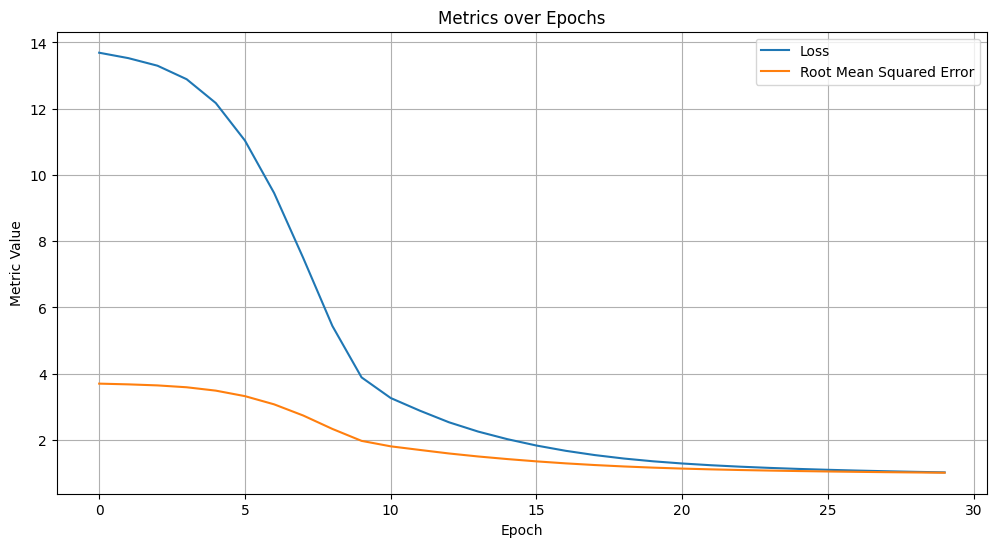
def plot_training_metrics(history):
    """Graphs all metrics tracked in the history object."""
    plt.figure(figsize=(12, 6))

    for metric_name, metric_values in history.history.items():
        plt.plot(metric_values, label=metric_name.replace("_", " ").title())

    plt.title("Metrics over Epochs")
    plt.xlabel("Epoch")
    plt.ylabel("Metric Value")
    plt.legend()
    plt.grid(True)


def visualize_layer(matrix, features, cmap=plt.cm.Blues):

    im = plt.matshow(
        matrix, cmap=cmap, extent=[-0.5, len(features) - 0.5, len(features) - 0.5, -0.5]
    )

    ax = plt.gca()
    divider = make_axes_locatable(plt.gca())
    cax = divider.append_axes("right", size="5%", pad=0.05)
    plt.colorbar(im, cax=cax)
    cax.tick_params(labelsize=10)

    # Set tick locations explicitly before setting labels
    ax.set_xticks(np.arange(len(features)))
    ax.set_yticks(np.arange(len(features)))

    ax.set_xticklabels(features, rotation=45, fontsize=5)
    ax.set_yticklabels(features, fontsize=5)

    plt.show()


def train_and_evaluate(
    learning_rate,
    epochs,
    train_data,
    test_data,
    model,
    plot_metrics=False,
):
    optimizer = keras.optimizers.AdamW(learning_rate=learning_rate, clipnorm=1.0)
    loss = keras.losses.MeanSquaredError()
    rmse = keras.metrics.RootMeanSquaredError()

    model.compile(
        optimizer=optimizer,
        loss=loss,
        metrics=[rmse],
    )

    history = model.fit(
        train_data,
        epochs=epochs,
        verbose=1,
    )
    if plot_metrics:
        plot_training_metrics(history)

    results = model.evaluate(test_data, return_dict=True, verbose=1)
    rmse_value = results["root_mean_squared_error"]

    return rmse_value, model.count_params()


def print_stats(rmse_list, num_params, model_name):
    # Report metrics.
    num_trials = len(rmse_list)
    avg_rmse = np.mean(rmse_list)
    std_rmse = np.std(rmse_list)

    if num_trials == 1:
        print(f"{model_name}: RMSE = {avg_rmse}; #params = {num_params}")
    else:
        print(f"{model_name}: RMSE = {avg_rmse} ± {std_rmse}; #params = {num_params}")

Real-world example

Let's use the MovieLens 100K dataset. This dataset is used to train models to predict users' movie ratings, based on user-related features and movie-related features.

Preparing the dataset

The dataset processing steps here are similar to what's given in the basic ranking tutorial. Let's load the dataset, and keep only the useful columns.

ratings_ds = tfds.load("movielens/100k-ratings", split="train")


def preprocess_features(x):
    """Extracts and cyclically encodes timestamp features."""
    features = {
        "movie_id": x["movie_id"],
        "user_id": x["user_id"],
        "user_gender": tf.cast(x["user_gender"], dtype=tf.int32),
        "user_zip_code": x["user_zip_code"],
        "user_occupation_text": x["user_occupation_text"],
        "raw_user_age": tf.cast(x["raw_user_age"], dtype=tf.float32),
    }
    label = tf.cast(x["user_rating"], dtype=tf.float32)

    # The timestamp is in seconds since the epoch.
    timestamp = tf.cast(x["timestamp"], dtype=tf.float32)

    # Constants for time periods
    SECONDS_IN_HOUR = 3600.0
    HOURS_IN_DAY = 24.0
    HOURS_IN_WEEK = 168.0

    # Calculate hour of day and encode it
    hour_of_day = (timestamp / SECONDS_IN_HOUR) % HOURS_IN_DAY
    features["hour_of_day_sin"] = tf.sin(2 * np.pi * hour_of_day / HOURS_IN_DAY)
    features["hour_of_day_cos"] = tf.cos(2 * np.pi * hour_of_day / HOURS_IN_DAY)

    # Calculate hour of week and encode it
    hour_of_week = (timestamp / SECONDS_IN_HOUR) % HOURS_IN_WEEK
    features["hour_of_week_sin"] = tf.sin(2 * np.pi * hour_of_week / HOURS_IN_WEEK)
    features["hour_of_week_cos"] = tf.cos(2 * np.pi * hour_of_week / HOURS_IN_WEEK)

    return features, label


# Apply the new preprocessing function
ratings_ds = ratings_ds.map(preprocess_features)

For every categorical feature, let's get the list of unique values, i.e., vocabulary, so that we can use that for the embedding layer.

vocabularies = {}
for feature_name in (
    MOVIELENS_CONFIG["categorical_int_features"]
    + MOVIELENS_CONFIG["categorical_str_features"]
):
    vocabulary = ratings_ds.batch(10_000).map(lambda x, y: x[feature_name])
    vocabularies[feature_name] = np.unique(np.concatenate(list(vocabulary)))

One thing we need to do is to use keras.layers.StringLookup and keras.layers.IntegerLookup to convert all the categorical features into indices, which can then be fed into embedding layers.

lookup_layers = {}
lookup_layers.update(
    {
        feature: keras.layers.IntegerLookup(vocabulary=vocabularies[feature])
        for feature in MOVIELENS_CONFIG["categorical_int_features"]
    }
)
lookup_layers.update(
    {
        feature: keras.layers.StringLookup(vocabulary=vocabularies[feature])
        for feature in MOVIELENS_CONFIG["categorical_str_features"]
    }
)

Let's normalize all the continuous features, so that we can use that for the MLP layers.

normalization_layers = {}
for feature_name in MOVIELENS_CONFIG["continuous_features"]:
    normalization_layers[feature_name] = keras.layers.Normalization(axis=-1)

training_data_for_adaptation = ratings_ds.take(80_000).map(lambda x, y: x)

for feature_name in MOVIELENS_CONFIG["continuous_features"]:
    feature_ds = training_data_for_adaptation.map(
        lambda x: tf.expand_dims(x[feature_name], axis=-1)
    )
    normalization_layers[feature_name].adapt(feature_ds)

ratings_ds = ratings_ds.map(
    lambda x, y: (
        {
            **{
                feature_name: lookup_layers[feature_name](x[feature_name])
                for feature_name in vocabularies
            },
            # Apply the adapted normalization layers to the continuous features.
            **{
                feature_name: tf.squeeze(
                    normalization_layers[feature_name](
                        tf.expand_dims(x[feature_name], axis=-1)
                    ),
                    axis=-1,
                )
                for feature_name in MOVIELENS_CONFIG["continuous_features"]
            },
        },
        y,
    )
)

Let's split our data into train and test sets. We also use cache() and prefetch() for better performance.

ratings_ds = ratings_ds.shuffle(100_000)

train_ds = (
    ratings_ds.take(80_000)
    .batch(MOVIELENS_CONFIG["batch_size"])
    .cache()
    .prefetch(tf.data.AUTOTUNE)
)
test_ds = (
    ratings_ds.skip(80_000)
    .batch(MOVIELENS_CONFIG["batch_size"])
    .take(20_000)
    .cache()
    .prefetch(tf.data.AUTOTUNE)
)

Building the model

The model will have embedding layers, followed by DotInteraction and feedforward layers.

class DLRM(keras.Model):
    def __init__(
        self,
        dense_num_units_lst,
        embedding_dim=MOVIELENS_CONFIG["embedding_dim"],
        mlp_dim=MOVIELENS_CONFIG["mlp_dim"],
        **kwargs,
    ):
        super().__init__(**kwargs)

        self.embedding_layers = {}
        for feature_name in (
            MOVIELENS_CONFIG["categorical_int_features"]
            + MOVIELENS_CONFIG["categorical_str_features"]
        ):
            vocab_size = len(vocabularies[feature_name]) + 1  # +1 for OOV token
            self.embedding_layers[feature_name] = keras.layers.Embedding(
                input_dim=vocab_size,
                output_dim=embedding_dim,
            )

        self.bottom_mlp = keras.Sequential(
            [
                keras.layers.Dense(mlp_dim, activation="relu"),
                keras.layers.Dense(embedding_dim),  # Output must match embedding_dim
            ]
        )

        self.dot_layer = keras_rs.layers.DotInteraction()

        self.top_mlp = []
        for num_units in dense_num_units_lst:
            self.top_mlp.append(keras.layers.Dense(num_units, activation="relu"))

        self.output_layer = keras.layers.Dense(1)

        self.dense_num_units_lst = dense_num_units_lst
        self.embedding_dim = embedding_dim

    def call(self, inputs):
        embeddings = []
        for feature_name in (
            MOVIELENS_CONFIG["categorical_int_features"]
            + MOVIELENS_CONFIG["categorical_str_features"]
        ):
            embedding = self.embedding_layers[feature_name](inputs[feature_name])
            embeddings.append(embedding)

        # Process all continuous features together.
        continuous_inputs = []
        for feature_name in MOVIELENS_CONFIG["continuous_features"]:
            # Reshape each feature to (batch_size, 1)
            feature = keras.ops.reshape(
                keras.ops.cast(inputs[feature_name], dtype="float32"), (-1, 1)
            )
            continuous_inputs.append(feature)

        # Concatenate into a single tensor: (batch_size, num_continuous_features)
        concatenated_continuous = keras.ops.concatenate(continuous_inputs, axis=1)

        # Pass through the Bottom MLP to get one combined vector.
        processed_continuous = self.bottom_mlp(concatenated_continuous)

        # Combine with categorical embeddings. Note: we add a list containing the
        # single tensor.
        combined_features = embeddings + [processed_continuous]

        # Pass the list of features to the DotInteraction layer.
        x = self.dot_layer(combined_features)

        for layer in self.top_mlp:
            x = layer(x)

        x = self.output_layer(x)

        return x


dot_network = DLRM(
    dense_num_units_lst=MOVIELENS_CONFIG["deep_net_num_units"],
    embedding_dim=MOVIELENS_CONFIG["embedding_dim"],
    mlp_dim=MOVIELENS_CONFIG["mlp_dim"],
)

rmse, dot_network_num_params = train_and_evaluate(
    learning_rate=MOVIELENS_CONFIG["learning_rate"],
    epochs=MOVIELENS_CONFIG["num_epochs"],
    train_data=train_ds,
    test_data=test_ds,
    model=dot_network,
    plot_metrics=True,
)
print_stats(
    rmse_list=[rmse],
    num_params=dot_network_num_params,
    model_name="Dot Network",
)

png

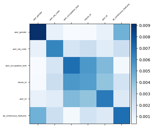
Visualizing feature interactions

The DotInteraction layer itself doesn't have a conventional "weight" matrix like a Dense layer. Instead, its function is to compute the dot product between the embedding vectors of your features.

To visualize the strength of these interactions, we can calculate a matrix representing the pairwise interaction strength between all feature embeddings. A common way to do this is to take the dot product of the embedding matrices for each pair of features and then aggregate the result into a single value (like the mean of the absolute values) that represents the overall interaction strength.

def get_dot_interaction_matrix(model, categorical_features, continuous_features):
    # The new feature list for the plot labels
    all_feature_names = categorical_features + ["all_continuous_features"]
    num_features = len(all_feature_names)

    # Store all feature outputs in the correct order.
    all_feature_outputs = []

    # Get outputs for categorical features from embedding layers (unchanged).
    for feature_name in categorical_features:
        embedding = model.embedding_layers[feature_name](keras.ops.array([0]))
        all_feature_outputs.append(embedding)

    # Get a single output for ALL continuous features from the shared MLP.
    num_continuous_features = len(continuous_features)
    # Create a dummy input of zeros for the MLP
    dummy_continuous_input = keras.ops.zeros((1, num_continuous_features))
    processed_continuous = model.bottom_mlp(dummy_continuous_input)
    all_feature_outputs.append(processed_continuous)

    interaction_matrix = np.zeros((num_features, num_features))

    # Iterate through each pair to calculate interaction strength.
    for i in range(num_features):
        for j in range(num_features):
            interaction = keras.ops.dot(
                all_feature_outputs[i], keras.ops.transpose(all_feature_outputs[j])
            )
            interaction_strength = keras.ops.convert_to_numpy(np.abs(interaction))[0][0]
            interaction_matrix[i, j] = interaction_strength

    return interaction_matrix, all_feature_names


# Get the list of categorical feature names.
categorical_feature_names = (
    MOVIELENS_CONFIG["categorical_int_features"]
    + MOVIELENS_CONFIG["categorical_str_features"]
)

# Calculate the interaction matrix with the corrected function.
interaction_matrix, feature_names = get_dot_interaction_matrix(
    model=dot_network,
    categorical_features=categorical_feature_names,
    continuous_features=MOVIELENS_CONFIG["continuous_features"],
)

# Visualize the matrix as a heatmap.
print("\nVisualizing the feature interaction strengths:")
visualize_layer(interaction_matrix, feature_names)