► KerasRS / Examples / Deep Recommenders

Deep Recommenders

Author: Fabien Hertschuh, Abheesht Sharma
Date created: 2025/04/28
Last modified: 2025/04/28
Description: Building a deep retrieval model with multiple stacked layers.

View in Colab • GitHub source

Introduction

One of the great advantages of using Keras to build recommender models is the freedom to build rich, flexible feature representations.

The first step in doing so is preparing the features, as raw features will usually not be immediately usable in a model.

For example: - User and item IDs may be strings (titles, usernames) or large, non-contiguous integers (database IDs). - Item descriptions could be raw text. - Interaction timestamps could be raw Unix timestamps.

These need to be appropriately transformed in order to be useful in building models: - User and item IDs have to be translated into embedding vectors, high-dimensional numerical representations that are adjusted during training to help the model predict its objective better. - Raw text needs to be tokenized (split into smaller parts such as individual words) and translated into embeddings. - Numerical features need to be normalized so that their values lie in a small interval around 0.

Fortunately, the Keras FeatureSpace utility makes this preprocessing easy.

In this tutorial, we are going to incorporate multiple features in our models. These features will come from preprocessing the MovieLens dataset.

In the basic retrieval tutorial, the models consist of only an embedding layer. In this tutorial, we add more dense layers to our models to increase their expressive power.

In general, deeper models are capable of learning more complex patterns than shallower models. For example, our user model incorporates user IDs and user features such as age, gender and occupation. A shallow model (say, a single embedding layer) may only be able to learn the simplest relationships between those features and movies: a given user generally prefers horror movies to comedies. To capture more complex relationships, such as user preferences evolving with their age, we may need a deeper model with multiple stacked dense layers.

Of course, complex models also have their disadvantages. The first is computational cost, as larger models require both more memory and more computation to train and serve. The second is the requirement for more data. In general, more training data is needed to take advantage of deeper models. With more parameters, deep models might overfit or even simply memorize the training examples instead of learning a function that can generalize. Finally, training deeper models may be harder, and more care needs to be taken in choosing settings like regularization and learning rate.

Finding a good architecture for a real-world recommender system is a complex art, requiring good intuition and careful hyperparameter tuning. For example, factors such as the depth and width of the model, activation function, learning rate, and optimizer can radically change the performance of the model. Modelling choices are further complicated by the fact that good offline evaluation metrics may not correspond to good online performance, and that the choice of what to optimize for is often more critical than the choice of model itself.

Nevertheless, effort put into building and fine-tuning larger models often pays off. In this tutorial, we will illustrate how to build a deep retrieval model. We'll do this by building progressively more complex models to see how this affects model performance.

import os

os.environ["KERAS_BACKEND"] = "jax"  # `"tensorflow"`/`"torch"`

import keras
import matplotlib.pyplot as plt
import tensorflow as tf  # Needed for the dataset
import tensorflow_datasets as tfds

import keras_rs

The MovieLens dataset

Let's first have a look at what features we can use from the MovieLens dataset.

# Ratings data with user and movie data.
ratings = tfds.load("movielens/100k-ratings", split="train")
# Features of all the available movies.
movies = tfds.load("movielens/100k-movies", split="train")

The ratings dataset returns a dictionary of movie id, user id, the assigned rating, timestamp, movie information, and user information:

for data in ratings.take(1).as_numpy_iterator():
    print(str(data).replace(", '", ",\n '"))

{'bucketized_user_age': np.float32(45.0),
 'movie_genres': array([7]),
 'movie_id': b'357',
 'movie_title': b"One Flew Over the Cuckoo's Nest (1975)",
 'raw_user_age': np.float32(46.0),
 'timestamp': np.int64(879024327),
 'user_gender': np.True_,
 'user_id': b'138',
 'user_occupation_label': np.int64(4),
 'user_occupation_text': b'doctor',
 'user_rating': np.float32(4.0),
 'user_zip_code': b'53211'}

In the Movielens dataset, user IDs are integers (represented as strings) starting at 1 and with no gap. Normally, you would need to create a lookup table to map user IDs to integers from 0 to N-1. But as a simplication, we'll use the user id directly as an index in our model, in particular to lookup the user embedding from the user embedding table. So we need do know the number of users.

USERS_COUNT = (
    ratings.map(lambda x: tf.strings.to_number(x["user_id"], out_type=tf.int32))
    .reduce(tf.constant(0, tf.int32), tf.maximum)
    .numpy()
)

The movies dataset contains the movie id, movie title, and the genres it belongs to. Note that the genres are encoded with integer labels.

for data in movies.take(1).as_numpy_iterator():
    print(str(data).replace(", '", ",\n '"))

{'movie_genres': array([4]),
 'movie_id': b'1681',
 'movie_title': b'You So Crazy (1994)'}

In the Movielens dataset, movie IDs are integers (represented as strings) starting at 1 and with no gap. Normally, you would need to create a lookup table to map movie IDs to integers from 0 to N-1. But as a simplication, we'll use the movie id directly as an index in our model, in particular to lookup the movie embedding from the movie embedding table. So we need do know the number of movies.

MOVIES_COUNT = movies.cardinality().numpy()

Preprocessing the dataset

Normalizing continuous features

Continuous features may need normalization so that they fall within an acceptable range for the model. We will give two examples of such normalization.

Discretization

A common transformation is to turn a continuous feature into a number of categorical features. This makes good sense if we have reasons to suspect that a feature's effect is non-continuous.

We need to decide on a number the buckets we will use for discretization. Then, we will use the Keras FeatureSpace utility to automatically find the minimum and maximum value, and divide that range by the number of buckets to perform the discretization.

In this example, we will discretize the user age.

AGE_BINS_COUNT = 10
user_age_feature = keras.utils.FeatureSpace.float_discretized(
    num_bins=AGE_BINS_COUNT, output_mode="int"
)

Rescaling

Often, we want continous features to be between 0 and 1, or between -1 and 1. To achieve this, we can rescale features that have a different range.

In this example, we will standardize the rating, which is a integer between 1 and 5, to be a float between 0 and 1. We need to rescale it and offset it.

user_rating_feature = keras.utils.FeatureSpace.float_rescaled(
    scale=1.0 / 4.0, offset=-1.0 / 4.0
)

Turning categorical features into embeddings

A categorical feature is a feature that does not express a continuous quantity, but rather takes on one of a set of fixed values.

Most deep learning models express these feature by turning them into high-dimensional vectors. During model training, the value of that vector is adjusted to help the model predict its objective better.

For example, suppose that our goal is to predict which user is going to watch which movie. To do that, we represent each user and each movie by an embedding vector. Initially, these embeddings will take on random values. During training, we adjust them so that embeddings of users and the movies they watch end up closer together.

Taking raw categorical features and turning them into embeddings is normally a two-step process: 1. First, we need to translate the raw values into a range of contiguous integers, normally by building a mapping (called a "vocabulary") that maps raw values to integers. 2. Second, we need to take these integers and turn them into embeddings.

Defining categorical features

We will use the Keras FeatureSpace utility for the first step. Its adapt method automatically discovers the vocabulary for categorical features.

user_gender_feature = keras.utils.FeatureSpace.integer_categorical(
    num_oov_indices=0, output_mode="int"
)
user_occupation_feature = keras.utils.FeatureSpace.integer_categorical(
    num_oov_indices=0, output_mode="int"
)

Using feature crosses

With crosses we can do feature interactions between multiple categorical features. This can be powerful to express that the combination of features represents a specific taste for movies.

Note that the combination of multiple features can result into on a super large feature space, that is why the crossing_dim parameter is important to limit the output dimension of the cross feature.

In this example, we will cross age and gender with the Keras FeatureSpace utility.

USER_GENDER_CROSS_COUNT = 20
user_gender_age_cross = keras.utils.FeatureSpace.cross(
    feature_names=("user_gender", "raw_user_age"),
    crossing_dim=USER_GENDER_CROSS_COUNT,
    output_mode="int",
)

Processing text features

We may also want to add text features to our model. Usually, things like product descriptions are free form text, and we can hope that our model can learn to use the information they contain to make better recommendations, especially in a cold-start or long tail scenario.

While the MovieLens dataset does not give us rich textual features, we can still use movie titles. This may help us capture the fact that movies with very similar titles are likely to belong to the same series.

The first transformation we need to apply to text is tokenization (splitting into constituent words or word-pieces), followed by vocabulary learning, followed by an embedding.

The [keras.layers.TextVectorization](/api/layers/preprocessing_layers/text/text_vectorization#textvectorization-class) layer can do the first two steps for us.

title_vectorizer = keras.layers.TextVectorization(
    max_tokens=10_000, output_sequence_length=16, dtype="int32"
)
title_vectorizer.adapt(movies.map(lambda x: x["movie_title"]))

Let's try it out:

for data in movies.take(1).as_numpy_iterator():
    print(title_vectorizer(data["movie_title"]))

[ 59 187 622   5   0   0   0   0   0   0   0   0   0   0   0   0]

Each title is translated into a sequence of tokens, one for each piece we've tokenized.

We can check the learned vocabulary to verify that the layer is using the correct tokenization:

print(title_vectorizer.get_vocabulary()[40:50])

[np.str_('paris'), np.str_('little'), np.str_('last'), np.str_('ii'), np.str_('1988'), np.str_('king'), np.str_('from'), np.str_('city'), np.str_('boys'), np.str_('murder')]

This looks correct, the layer is tokenizing titles into individual words. Later, we will see how to embed this tokenized text. For now, we turn this vectorizer into a Keras FeatureSpace feature.

title_feature = keras.utils.FeatureSpace.feature(
    preprocessor=title_vectorizer, dtype="string", output_mode="float"
)
TITLE_TOKEN_COUNT = title_vectorizer.vocabulary_size()

Putting the FeatureSpace features together

We're now ready to assemble the features with preprocessors in a FeatureSpace object. We're then using adapt to go through the dataset and learn what needs to be learned, such as the vocabulary size for categorical features or the minimum and maximum values for bucketized features.

feature_space = keras.utils.FeatureSpace(
    features={
        # Numerical features to discretize.
        "raw_user_age": user_age_feature,
        # Categorical features encoded as integers.
        "user_gender": user_gender_feature,
        "user_occupation_label": user_occupation_feature,
        # Labels are ratings between 0 and 1.
        "user_rating": user_rating_feature,
        "movie_title": title_feature,
    },
    crosses=[user_gender_age_cross],
    output_mode="dict",
)

feature_space.adapt(ratings)
GENDERS_COUNT = feature_space.preprocessors["user_gender"].vocabulary_size()
OCCUPATIONS_COUNT = feature_space.preprocessors[
    "user_occupation_label"
].vocabulary_size()

Pre-building the candidate set

Our model is going to based on a Retrieval layer, which can provides a set of best candidates among to full set of candidates. To do this, the retrieval layer needs to know all the candidates and their features. In this section, we assemble the full set of movies with the associated features.

Extract raw candidate features

First, we gather all the raw features from the dataset in lists. That is the titles of the movies and the genres. Note that one or more genres are associated with each movie, and the number of genres varies per movie.

movie_titles = [""] * (MOVIES_COUNT + 1)
movie_genres = [[]] * (MOVIES_COUNT + 1)
for x in movies.as_numpy_iterator():
    movie_id = int(x["movie_id"])
    movie_titles[movie_id] = x["movie_title"]
    movie_genres[movie_id] = x["movie_genres"].tolist()

Preprocess candidate features

Genres are already in the form of category numbers starting at zero. However, we do need to figure out two things: - The maximum number of genres a single movie can have; this will determine the dimension for this feature. - The maximum value for the genre, which will give us the total number of genres and determine the size of our embedding table for genres.

MAX_GENRES_PER_MOVIE = 0
max_genre_id = 0
for one_movie_genres in movie_genres:
    MAX_GENRES_PER_MOVIE = max(MAX_GENRES_PER_MOVIE, len(one_movie_genres))
    if one_movie_genres:
        max_genre_id = max(max_genre_id, max(one_movie_genres))

GENRES_COUNT = max_genre_id + 1

Now we need to pad genres with an Out Of Vocabulary value to be able to represent genres as a fixed size vector. We'll pad with zeros for simplicity, so we're adding one to the genres to not conflict with genre zero, which is a valid genre.

movie_genres = [
    [g + 1 for g in genres] + [0] * (MAX_GENRES_PER_MOVIE - len(genres))
    for genres in movie_genres
]

Then, we vectorize all the movie titles.

movie_titles_vectors = title_vectorizer(movie_titles)

Convert candidate set to native tensors

We're now ready to combine these in a dataset. The last step is to make sure everything is a native tensor that can be consumed by the retrieval layer. As a remminder, movie id zero does not exist.

MOVIES_DATASET = {
    "movie_id": keras.ops.arange(0, MOVIES_COUNT + 1, dtype="int32"),
    "movie_title_vector": movie_titles_vectors,
    "movie_genres": keras.ops.convert_to_tensor(movie_genres, dtype="int32"),
}

Preparing the data

We can now define our preprocessing function. Most features will be handled by the FeatureSpace. User IDs and Movie IDs need to be extracted. Movie genres need to be padded. Then everything is packaged as a tuple with a dict of input features and a float for the rating, which is used as a label.

def preprocess_rating(x):
    features = feature_space(
        {
            "raw_user_age": x["raw_user_age"],
            "user_gender": x["user_gender"],
            "user_occupation_label": x["user_occupation_label"],
            "user_rating": x["user_rating"],
            "movie_title": x["movie_title"],
        }
    )
    features = {k: tf.squeeze(v, axis=0) for k, v in features.items()}
    movie_genres = x["movie_genres"]

    return (
        {
            # User inputs are user ID and user features
            "user_id": int(x["user_id"]),
            "raw_user_age": features["raw_user_age"],
            "user_gender": features["user_gender"],
            "user_occupation_label": features["user_occupation_label"],
            "user_gender_X_raw_user_age": features["user_gender_X_raw_user_age"],
            # Movie inputs are movie ID, vectorized title and genres
            "movie_id": int(x["movie_id"]),
            "movie_title_vector": features["movie_title"],
            "movie_genres": tf.pad(
                movie_genres + 1,
                [[0, MAX_GENRES_PER_MOVIE - tf.shape(movie_genres)[0]]],
            ),
        },
        # Label is user rating between 0 and 1
        features["user_rating"],
    )

We shuffle and then split the data into a training set and a testing set.

shuffled_ratings = ratings.map(preprocess_rating).shuffle(
    100_000, seed=42, reshuffle_each_iteration=False
)

train_ratings = shuffled_ratings.take(80_000).batch(1000).cache()
test_ratings = shuffled_ratings.skip(80_000).take(20_000).batch(1000).cache()

Model definition

Query model

The query model is first tasked with converting user features to embeddings. The embeddings are then concatenated into a single vector.

Defining deeper models will require us to stack more layers on top of this first set of embeddings. A progressively narrower stack of layers, separated by an activation function, is a common pattern:

                            +----------------------+
                            |       64 x 32        |
                            +----------------------+
                                       | relu
                          +--------------------------+
                          |         128 x 64         |
                          +--------------------------+
                                       | relu
                        +------------------------------+
                        |          ... x 128           |
                        +------------------------------+

Since the expressive power of deep linear models is no greater than that of shallow linear models, we use ReLU activations for all but the last hidden layer. The final hidden layer does not use any activation function: using an activation function would limit the output space of the final embeddings and might negatively impact the performance of the model. For instance, if ReLUs are used in the projection layer, all components in the output embedding would be non-negative.

We're going to try this here. To make experimentation with different depths easy, let's define a model whose depth (and width) is defined by a constructor parameters. The layer_sizes parameter gives us the depth and width of the model. We can vary it to experiment with shallower or deeper models.

class QueryModel(keras.Model):
    """Model for encoding user queries."""

    def __init__(self, layer_sizes, embedding_dimension=32):
        """Construct a model for encoding user queries.

        Args:
          layer_sizes: A list of integers where the i-th entry represents the
            number of units the i-th layer contains.
          embedding_dimension: Output dimension for all embedding tables.
        """
        super().__init__()

        # We first generate embeddings.
        self.user_embedding = keras.layers.Embedding(
            # +1 for user ID zero, which does not exist
            USERS_COUNT + 1,
            embedding_dimension,
        )
        self.gender_embedding = keras.layers.Embedding(
            GENDERS_COUNT, embedding_dimension
        )
        self.age_embedding = keras.layers.Embedding(AGE_BINS_COUNT, embedding_dimension)
        self.gender_x_age_embedding = keras.layers.Embedding(
            USER_GENDER_CROSS_COUNT, embedding_dimension
        )
        self.occupation_embedding = keras.layers.Embedding(
            OCCUPATIONS_COUNT, embedding_dimension
        )

        # Then construct the layers.
        self.dense_layers = keras.Sequential()

        # Use the ReLU activation for all but the last layer.
        for layer_size in layer_sizes[:-1]:
            self.dense_layers.add(keras.layers.Dense(layer_size, activation="relu"))

        # No activation for the last layer.
        self.dense_layers.add(keras.layers.Dense(layer_sizes[-1]))

    def call(self, inputs):
        # Take the inputs, pass each through its embedding layer, concatenate.
        feature_embedding = keras.ops.concatenate(
            [
                self.user_embedding(inputs["user_id"]),
                self.gender_embedding(inputs["user_gender"]),
                self.age_embedding(inputs["raw_user_age"]),
                self.gender_x_age_embedding(inputs["user_gender_X_raw_user_age"]),
                self.occupation_embedding(inputs["user_occupation_label"]),
            ],
            axis=1,
        )
        return self.dense_layers(feature_embedding)

Candidate model

We can adopt the same approach for the candidate model. Again, we start with converting movie features to embeddings, concatenate them and then expand it with hidden layers:

class CandidateModel(keras.Model):
    """Model for encoding candidates (movies)."""

    def __init__(self, layer_sizes, embedding_dimension=32):
        """Construct a model for encoding candidates (movies).

        Args:
          layer_sizes: A list of integers where the i-th entry represents the
            number of units the i-th layer contains.
          embedding_dimension: Output dimension for all embedding tables.
        """
        super().__init__()

        # We first generate embeddings.
        self.movie_embedding = keras.layers.Embedding(
            # +1 for movie ID zero, which does not exist
            MOVIES_COUNT + 1,
            embedding_dimension,
        )
        # Take all the title tokens for the title of the movie, embed each
        # token, and then take the mean of all token embeddings.
        self.movie_title_embedding = keras.Sequential(
            [
                keras.layers.Embedding(
                    # +1 for OOV token, which is used for padding
                    TITLE_TOKEN_COUNT + 1,
                    embedding_dimension,
                    mask_zero=True,
                ),
                keras.layers.GlobalAveragePooling1D(),
            ]
        )
        # Take all the genres for the movie, embed each genre, and then take the
        # mean of all genre embeddings.
        self.movie_genres_embedding = keras.Sequential(
            [
                keras.layers.Embedding(
                    # +1 for OOV genre, which is used for padding
                    GENRES_COUNT + 1,
                    embedding_dimension,
                    mask_zero=True,
                ),
                keras.layers.GlobalAveragePooling1D(),
            ]
        )

        # Then construct the layers.
        self.dense_layers = keras.Sequential()

        # Use the ReLU activation for all but the last layer.
        for layer_size in layer_sizes[:-1]:
            self.dense_layers.add(keras.layers.Dense(layer_size, activation="relu"))

        # No activation for the last layer.
        self.dense_layers.add(keras.layers.Dense(layer_sizes[-1]))

    def call(self, inputs):
        movie_id = inputs["movie_id"]
        movie_title_vector = inputs["movie_title_vector"]
        movie_genres = inputs["movie_genres"]
        feature_embedding = keras.ops.concatenate(
            [
                self.movie_embedding(movie_id),
                self.movie_title_embedding(movie_title_vector),
                self.movie_genres_embedding(movie_genres),
            ],
            axis=1,
        )
        return self.dense_layers(feature_embedding)

Combined model

With both QueryModel and CandidateModel defined, we can put together a combined model and implement our loss and metrics logic. To make things simple, we'll enforce that the model structure is the same across the query and candidate models.

class RetrievalModel(keras.Model):
    """Combined model."""

    def __init__(
        self,
        layer_sizes=(32,),
        embedding_dimension=32,
        retrieval_k=100,
    ):
        """Construct a combined model.

        Args:
          layer_sizes: A list of integers where the i-th entry represents the
            number of units the i-th layer contains.
          embedding_dimension: Output dimension for all embedding tables.
          retrieval_k: How many candidate movies to retrieve.
        """
        super().__init__()
        self.query_model = QueryModel(layer_sizes, embedding_dimension)
        self.candidate_model = CandidateModel(layer_sizes, embedding_dimension)
        self.retrieval = keras_rs.layers.BruteForceRetrieval(
            k=retrieval_k, return_scores=False
        )
        self.update_candidates()  # Provide an initial set of candidates
        self.loss_fn = keras.losses.MeanSquaredError()
        self.top_k_metric = keras.metrics.SparseTopKCategoricalAccuracy(
            k=retrieval_k, from_sorted_ids=True
        )

    def update_candidates(self):
        self.retrieval.update_candidates(
            self.candidate_model.predict(MOVIES_DATASET, verbose=0)
        )

    def call(self, inputs, training=False):
        query_embeddings = self.query_model(
            {
                "user_id": inputs["user_id"],
                "raw_user_age": inputs["raw_user_age"],
                "user_gender": inputs["user_gender"],
                "user_occupation_label": inputs["user_occupation_label"],
                "user_gender_X_raw_user_age": inputs["user_gender_X_raw_user_age"],
            }
        )
        candidate_embeddings = self.candidate_model(
            {
                "movie_id": inputs["movie_id"],
                "movie_title_vector": inputs["movie_title_vector"],
                "movie_genres": inputs["movie_genres"],
            }
        )

        result = {
            "query_embeddings": query_embeddings,
            "candidate_embeddings": candidate_embeddings,
        }
        if not training:
            # No need to spend time extracting top predicted movies during
            # training, they are not used.
            result["predictions"] = self.retrieval(query_embeddings)
        return result

    def evaluate(
        self,
        x=None,
        y=None,
        batch_size=None,
        verbose="auto",
        sample_weight=None,
        steps=None,
        callbacks=None,
        return_dict=False,
        **kwargs,
    ):
        """Overridden to update the candidate set.

        Before evaluating the model, we need to update our retrieval layer by
        re-computing the values predicted by the candidate model for all the
        candidates.
        """
        self.update_candidates()
        return super().evaluate(
            x,
            y,
            batch_size=batch_size,
            verbose=verbose,
            sample_weight=sample_weight,
            steps=steps,
            callbacks=callbacks,
            return_dict=return_dict,
            **kwargs,
        )

    def compute_loss(self, x, y, y_pred, sample_weight, training=True):
        query_embeddings = y_pred["query_embeddings"]
        candidate_embeddings = y_pred["candidate_embeddings"]

        labels = keras.ops.expand_dims(y, -1)
        # Compute the affinity score by multiplying the two embeddings.
        scores = keras.ops.sum(
            keras.ops.multiply(query_embeddings, candidate_embeddings),
            axis=1,
            keepdims=True,
        )
        return self.loss_fn(labels, scores, sample_weight)

    def compute_metrics(self, x, y, y_pred, sample_weight=None):
        if "predictions" in y_pred:
            # We are evaluating or predicting. Update `top_k_metric`.
            movie_ids = x["movie_id"]
            predictions = y_pred["predictions"]
            # For `top_k_metric`, which is a `SparseTopKCategoricalAccuracy`, we
            # only take top rated movies, and we put a weight of 0 for the rest.
            rating_weight = keras.ops.cast(keras.ops.greater(y, 0.9), "float32")
            sample_weight = (
                rating_weight
                if sample_weight is None
                else keras.ops.multiply(rating_weight, sample_weight)
            )
            self.top_k_metric.update_state(
                movie_ids, predictions, sample_weight=sample_weight
            )
            return self.get_metrics_result()
        else:
            # We are training. `top_k_metric` is not updated and is zero, so
            # don't report it.
            result = self.get_metrics_result()
            result.pop(self.top_k_metric.name)
            return result

Training the model

Shallow model

We're ready to try out our first, shallow, model!

NUM_EPOCHS = 30

one_layer_model = RetrievalModel((32,))
one_layer_model.compile(optimizer=keras.optimizers.Adagrad(0.05))

one_layer_history = one_layer_model.fit(
    train_ratings,
    validation_data=test_ratings,
    validation_freq=5,
    epochs=NUM_EPOCHS,
)

Epoch 1/30
80/80 ━━━━━━━━━━━━━━━━━━━━ 19s 18ms/step - loss: 0.2392
Epoch 2/30
80/80 ━━━━━━━━━━━━━━━━━━━━ 1s 4ms/step - loss: 0.0764
Epoch 3/30
80/80 ━━━━━━━━━━━━━━━━━━━━ 0s 4ms/step - loss: 0.0748
Epoch 4/30
80/80 ━━━━━━━━━━━━━━━━━━━━ 0s 4ms/step - loss: 0.0737
Epoch 5/30
80/80 ━━━━━━━━━━━━━━━━━━━━ 19s 242ms/step - loss: 0.0727 - val_loss: 0.0736 - val_sparse_top_k_categorical_accuracy: 0.1196
Epoch 6/30
80/80 ━━━━━━━━━━━━━━━━━━━━ 0s 4ms/step - loss: 0.0718
Epoch 7/30
80/80 ━━━━━━━━━━━━━━━━━━━━ 0s 4ms/step - loss: 0.0710
Epoch 8/30
80/80 ━━━━━━━━━━━━━━━━━━━━ 0s 4ms/step - loss: 0.0702
Epoch 9/30
80/80 ━━━━━━━━━━━━━━━━━━━━ 0s 4ms/step - loss: 0.0694
Epoch 10/30
80/80 ━━━━━━━━━━━━━━━━━━━━ 0s 6ms/step - loss: 0.0685 - val_loss: 0.0695 - val_sparse_top_k_categorical_accuracy: 0.2117
Epoch 11/30
80/80 ━━━━━━━━━━━━━━━━━━━━ 0s 4ms/step - loss: 0.0677
Epoch 12/30
80/80 ━━━━━━━━━━━━━━━━━━━━ 0s 4ms/step - loss: 0.0669
Epoch 13/30
80/80 ━━━━━━━━━━━━━━━━━━━━ 0s 4ms/step - loss: 0.0661
Epoch 14/30
80/80 ━━━━━━━━━━━━━━━━━━━━ 0s 4ms/step - loss: 0.0653
Epoch 15/30
80/80 ━━━━━━━━━━━━━━━━━━━━ 0s 6ms/step - loss: 0.0645 - val_loss: 0.0655 - val_sparse_top_k_categorical_accuracy: 0.2742
Epoch 16/30
80/80 ━━━━━━━━━━━━━━━━━━━━ 0s 4ms/step - loss: 0.0637
Epoch 17/30
80/80 ━━━━━━━━━━━━━━━━━━━━ 0s 4ms/step - loss: 0.0629
Epoch 18/30
80/80 ━━━━━━━━━━━━━━━━━━━━ 0s 4ms/step - loss: 0.0622
Epoch 19/30
80/80 ━━━━━━━━━━━━━━━━━━━━ 0s 4ms/step - loss: 0.0615
Epoch 20/30
80/80 ━━━━━━━━━━━━━━━━━━━━ 0s 6ms/step - loss: 0.0608 - val_loss: 0.0621 - val_sparse_top_k_categorical_accuracy: 0.2994
Epoch 21/30
80/80 ━━━━━━━━━━━━━━━━━━━━ 0s 4ms/step - loss: 0.0602
Epoch 22/30
80/80 ━━━━━━━━━━━━━━━━━━━━ 0s 4ms/step - loss: 0.0596
Epoch 23/30
80/80 ━━━━━━━━━━━━━━━━━━━━ 0s 4ms/step - loss: 0.0590
Epoch 24/30
80/80 ━━━━━━━━━━━━━━━━━━━━ 0s 4ms/step - loss: 0.0585
Epoch 25/30
80/80 ━━━━━━━━━━━━━━━━━━━━ 0s 6ms/step - loss: 0.0580 - val_loss: 0.0596 - val_sparse_top_k_categorical_accuracy: 0.3150
Epoch 26/30
80/80 ━━━━━━━━━━━━━━━━━━━━ 0s 4ms/step - loss: 0.0576
Epoch 27/30
80/80 ━━━━━━━━━━━━━━━━━━━━ 0s 4ms/step - loss: 0.0572
Epoch 28/30
80/80 ━━━━━━━━━━━━━━━━━━━━ 0s 4ms/step - loss: 0.0569
Epoch 29/30
80/80 ━━━━━━━━━━━━━━━━━━━━ 0s 4ms/step - loss: 0.0565
Epoch 30/30
80/80 ━━━━━━━━━━━━━━━━━━━━ 1s 7ms/step - loss: 0.0562 - val_loss: 0.0581 - val_sparse_top_k_categorical_accuracy: 0.3100

This gives us a top-100 accuracy of around 0.30. We can use this as a reference point for evaluating deeper models.

Deeper model

What about a deeper model with two layers?

two_layer_model = RetrievalModel((64, 32))
two_layer_model.compile(optimizer=keras.optimizers.Adagrad(0.05))
two_layer_history = two_layer_model.fit(
    train_ratings,
    validation_data=test_ratings,
    validation_freq=5,
    epochs=NUM_EPOCHS,
)

Epoch 1/30
80/80 ━━━━━━━━━━━━━━━━━━━━ 2s 15ms/step - loss: 0.2066
Epoch 2/30
80/80 ━━━━━━━━━━━━━━━━━━━━ 1s 4ms/step - loss: 0.0756
Epoch 3/30
80/80 ━━━━━━━━━━━━━━━━━━━━ 0s 4ms/step - loss: 0.0736
Epoch 4/30
80/80 ━━━━━━━━━━━━━━━━━━━━ 0s 4ms/step - loss: 0.0721
Epoch 5/30
80/80 ━━━━━━━━━━━━━━━━━━━━ 2s 25ms/step - loss: 0.0708 - val_loss: 0.0713 - val_sparse_top_k_categorical_accuracy: 0.1530
Epoch 6/30
80/80 ━━━━━━━━━━━━━━━━━━━━ 0s 4ms/step - loss: 0.0696
Epoch 7/30
80/80 ━━━━━━━━━━━━━━━━━━━━ 0s 4ms/step - loss: 0.0685
Epoch 8/30
80/80 ━━━━━━━━━━━━━━━━━━━━ 1s 8ms/step - loss: 0.0675
Epoch 9/30
80/80 ━━━━━━━━━━━━━━━━━━━━ 0s 4ms/step - loss: 0.0664
Epoch 10/30
80/80 ━━━━━━━━━━━━━━━━━━━━ 1s 6ms/step - loss: 0.0654 - val_loss: 0.0661 - val_sparse_top_k_categorical_accuracy: 0.2355
Epoch 11/30
80/80 ━━━━━━━━━━━━━━━━━━━━ 0s 4ms/step - loss: 0.0644
Epoch 12/30
80/80 ━━━━━━━━━━━━━━━━━━━━ 0s 4ms/step - loss: 0.0634
Epoch 13/30
80/80 ━━━━━━━━━━━━━━━━━━━━ 0s 4ms/step - loss: 0.0625
Epoch 14/30
80/80 ━━━━━━━━━━━━━━━━━━━━ 0s 4ms/step - loss: 0.0616
Epoch 15/30
80/80 ━━━━━━━━━━━━━━━━━━━━ 0s 6ms/step - loss: 0.0608 - val_loss: 0.0618 - val_sparse_top_k_categorical_accuracy: 0.2882
Epoch 16/30
80/80 ━━━━━━━━━━━━━━━━━━━━ 0s 4ms/step - loss: 0.0600
Epoch 17/30
80/80 ━━━━━━━━━━━━━━━━━━━━ 0s 4ms/step - loss: 0.0594
Epoch 18/30
80/80 ━━━━━━━━━━━━━━━━━━━━ 0s 4ms/step - loss: 0.0587
Epoch 19/30
80/80 ━━━━━━━━━━━━━━━━━━━━ 0s 4ms/step - loss: 0.0582
Epoch 20/30
80/80 ━━━━━━━━━━━━━━━━━━━━ 1s 10ms/step - loss: 0.0577 - val_loss: 0.0591 - val_sparse_top_k_categorical_accuracy: 0.3072
Epoch 21/30
80/80 ━━━━━━━━━━━━━━━━━━━━ 0s 4ms/step - loss: 0.0573
Epoch 22/30
80/80 ━━━━━━━━━━━━━━━━━━━━ 0s 4ms/step - loss: 0.0569
Epoch 23/30
80/80 ━━━━━━━━━━━━━━━━━━━━ 0s 4ms/step - loss: 0.0566
Epoch 24/30
80/80 ━━━━━━━━━━━━━━━━━━━━ 0s 4ms/step - loss: 0.0562
Epoch 25/30
80/80 ━━━━━━━━━━━━━━━━━━━━ 0s 6ms/step - loss: 0.0560 - val_loss: 0.0577 - val_sparse_top_k_categorical_accuracy: 0.3134
Epoch 26/30
80/80 ━━━━━━━━━━━━━━━━━━━━ 0s 4ms/step - loss: 0.0557
Epoch 27/30
80/80 ━━━━━━━━━━━━━━━━━━━━ 0s 4ms/step - loss: 0.0555
Epoch 28/30
80/80 ━━━━━━━━━━━━━━━━━━━━ 0s 4ms/step - loss: 0.0553
Epoch 29/30
80/80 ━━━━━━━━━━━━━━━━━━━━ 0s 4ms/step - loss: 0.0551
Epoch 30/30
80/80 ━━━━━━━━━━━━━━━━━━━━ 1s 6ms/step - loss: 0.0549 - val_loss: 0.0569 - val_sparse_top_k_categorical_accuracy: 0.3093

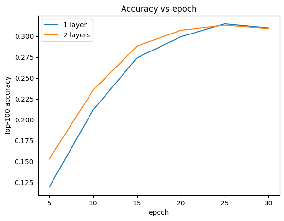
While the deeper model seems to learn a bit better than the shallow model at first, the difference becomes minimal towards the end of the trainign. We can plot the validation accuracy curves to illustrate this:

METRIC = "val_sparse_top_k_categorical_accuracy"
num_validation_runs = len(one_layer_history.history[METRIC])
epochs = [(x + 1) * 5 for x in range(num_validation_runs)]

plt.plot(epochs, one_layer_history.history[METRIC], label="1 layer")
plt.plot(epochs, two_layer_history.history[METRIC], label="2 layers")
plt.title("Accuracy vs epoch")
plt.xlabel("epoch")
plt.ylabel("Top-100 accuracy")
plt.legend()
plt.show()

png

Deeper models are not necessarily better. The following model extends the depth to three layers:

three_layer_model = RetrievalModel((128, 64, 32))
three_layer_model.compile(optimizer=keras.optimizers.Adagrad(0.05))
three_layer_history = three_layer_model.fit(
    train_ratings,
    validation_data=test_ratings,
    validation_freq=5,
    epochs=NUM_EPOCHS,
)

Epoch 1/30
80/80 ━━━━━━━━━━━━━━━━━━━━ 3s 17ms/step - loss: 0.1880
Epoch 2/30
80/80 ━━━━━━━━━━━━━━━━━━━━ 1s 4ms/step - loss: 0.0751
Epoch 3/30
80/80 ━━━━━━━━━━━━━━━━━━━━ 0s 4ms/step - loss: 0.0734
Epoch 4/30
80/80 ━━━━━━━━━━━━━━━━━━━━ 0s 4ms/step - loss: 0.0720
Epoch 5/30
80/80 ━━━━━━━━━━━━━━━━━━━━ 2s 26ms/step - loss: 0.0707 - val_loss: 0.0712 - val_sparse_top_k_categorical_accuracy: 0.1276
Epoch 6/30
80/80 ━━━━━━━━━━━━━━━━━━━━ 0s 4ms/step - loss: 0.0694
Epoch 7/30
80/80 ━━━━━━━━━━━━━━━━━━━━ 0s 5ms/step - loss: 0.0682
Epoch 8/30
80/80 ━━━━━━━━━━━━━━━━━━━━ 0s 4ms/step - loss: 0.0670
Epoch 9/30
80/80 ━━━━━━━━━━━━━━━━━━━━ 0s 4ms/step - loss: 0.0659
Epoch 10/30
80/80 ━━━━━━━━━━━━━━━━━━━━ 1s 6ms/step - loss: 0.0648 - val_loss: 0.0656 - val_sparse_top_k_categorical_accuracy: 0.2552
Epoch 11/30
80/80 ━━━━━━━━━━━━━━━━━━━━ 0s 5ms/step - loss: 0.0637
Epoch 12/30
80/80 ━━━━━━━━━━━━━━━━━━━━ 0s 4ms/step - loss: 0.0628
Epoch 13/30
80/80 ━━━━━━━━━━━━━━━━━━━━ 0s 4ms/step - loss: 0.0618
Epoch 14/30
80/80 ━━━━━━━━━━━━━━━━━━━━ 0s 4ms/step - loss: 0.0610
Epoch 15/30
80/80 ━━━━━━━━━━━━━━━━━━━━ 1s 6ms/step - loss: 0.0603 - val_loss: 0.0616 - val_sparse_top_k_categorical_accuracy: 0.2816
Epoch 16/30
80/80 ━━━━━━━━━━━━━━━━━━━━ 0s 4ms/step - loss: 0.0596
Epoch 17/30
80/80 ━━━━━━━━━━━━━━━━━━━━ 0s 4ms/step - loss: 0.0590
Epoch 18/30
80/80 ━━━━━━━━━━━━━━━━━━━━ 0s 4ms/step - loss: 0.0584
Epoch 19/30
80/80 ━━━━━━━━━━━━━━━━━━━━ 0s 4ms/step - loss: 0.0579
Epoch 20/30
80/80 ━━━━━━━━━━━━━━━━━━━━ 1s 7ms/step - loss: 0.0575 - val_loss: 0.0592 - val_sparse_top_k_categorical_accuracy: 0.2921
Epoch 21/30
80/80 ━━━━━━━━━━━━━━━━━━━━ 0s 4ms/step - loss: 0.0571
Epoch 22/30
80/80 ━━━━━━━━━━━━━━━━━━━━ 0s 4ms/step - loss: 0.0567
Epoch 23/30
80/80 ━━━━━━━━━━━━━━━━━━━━ 0s 4ms/step - loss: 0.0564
Epoch 24/30
80/80 ━━━━━━━━━━━━━━━━━━━━ 0s 4ms/step - loss: 0.0561
Epoch 25/30
80/80 ━━━━━━━━━━━━━━━━━━━━ 1s 6ms/step - loss: 0.0559 - val_loss: 0.0578 - val_sparse_top_k_categorical_accuracy: 0.2983
Epoch 26/30
80/80 ━━━━━━━━━━━━━━━━━━━━ 0s 4ms/step - loss: 0.0557
Epoch 27/30
80/80 ━━━━━━━━━━━━━━━━━━━━ 0s 5ms/step - loss: 0.0555
Epoch 28/30
80/80 ━━━━━━━━━━━━━━━━━━━━ 0s 4ms/step - loss: 0.0553
Epoch 29/30
80/80 ━━━━━━━━━━━━━━━━━━━━ 0s 4ms/step - loss: 0.0551
Epoch 30/30
80/80 ━━━━━━━━━━━━━━━━━━━━ 1s 6ms/step - loss: 0.0549 - val_loss: 0.0571 - val_sparse_top_k_categorical_accuracy: 0.3006

We don't really see an improvement over the shallow model:

plt.plot(epochs, one_layer_history.history[METRIC], label="1 layer")
plt.plot(epochs, two_layer_history.history[METRIC], label="2 layers")
plt.plot(epochs, three_layer_history.history[METRIC], label="3 layers")
plt.title("Accuracy vs epoch")
plt.xlabel("epoch")
plt.ylabel("Top-100 accuracy")
plt.legend()
plt.show()

png

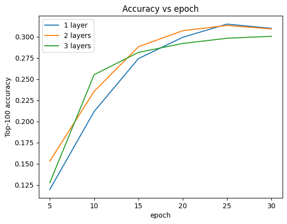
This is a good illustration of the fact that deeper and larger models, while capable of superior performance, often require very careful tuning. For example, throughout this tutorial we used a single, fixed learning rate. Alternative choices may give very different results and are worth exploring.

With appropriate tuning and sufficient data, the effort put into building larger and deeper models is in many cases well worth it: larger models can lead to substantial improvements in prediction accuracy.

Next Steps

In this tutorial we expanded our retrieval model with dense layers and activation functions. To see how to create a model that can perform not only retrieval tasks but also rating tasks, take a look at the multitask tutorial.