► KerasRS / Examples / Ranking with Deep and Cross Networks

Ranking with Deep and Cross Networks

Author: Abheesht Sharma, Fabien Hertschuh
Date created: 2025/04/28
Last modified: 2025/04/28
Description: Rank movies using Deep and Cross Networks (DCN).

View in Colab • GitHub source

Introduction

This tutorial demonstrates how to use Deep & Cross Networks (DCN) to effectively learn feature crosses. Before diving into the example, let's briefly discuss feature crosses.

Imagine that we are building a recommender system for blenders. Individual features might include a customer's past purchase history (e.g., purchased_bananas, purchased_cooking_books) or geographic location. However, a customer who has purchased both bananas and cooking books is more likely to be interested in a blender than someone who purchased only one or the other. The combination of purchased_bananas and purchased_cooking_books is a feature cross. Feature crosses capture interaction information between individual features, providing richer context than the individual features alone.

Why are feature crosses important?

Learning effective feature crosses presents several challenges. In web-scale applications, data is often categorical, resulting in high-dimensional and sparse feature spaces. Identifying impactful feature crosses in such environments typically relies on manual feature engineering or computationally expensive exhaustive searches. While traditional feed-forward multilayer perceptrons (MLPs) are universal function approximators, they often struggle to efficiently learn even second- or third-order feature interactions.

The Deep & Cross Network (DCN) architecture is designed for more effective learning of explicit and bounded-degree feature crosses. It comprises three main components: an input layer (typically an embedding layer), a cross network for modeling explicit feature interactions, and a deep network for capturing implicit interactions.

The cross network is the core of the DCN. It explicitly performs feature crossing at each layer, with the highest polynomial degree of feature interaction increasing with depth. The following figure shows the (i+1)-th cross layer.

Feature Cross Layer

The deep network is a standard feedforward multilayer perceptron (MLP). These two networks are then combined to form the DCN. Two common combination strategies exist: a stacked structure, where the deep network is placed on top of the cross network, and a parallel structure, where they operate in parallel.

Now that we know a little bit about DCN, let's start writing some code. We will first train a DCN on a toy dataset, and demonstrate that the model has indeed learnt important feature crosses.

Let's set the backend to JAX, and get our imports sorted.

import os

os.environ["KERAS_BACKEND"] = "jax"  # `"tensorflow"`/`"torch"`

import keras
import matplotlib.pyplot as plt
import numpy as np
import tensorflow as tf
import tensorflow_datasets as tfds
from mpl_toolkits.axes_grid1 import make_axes_locatable

import keras_rs

Let's also define variables which will be reused throughout the example.

TOY_CONFIG = {
    "learning_rate": 0.01,
    "num_epochs": 100,
    "batch_size": 1024,
}

MOVIELENS_CONFIG = {
    # features
    "int_features": [
        "movie_id",
        "user_id",
        "user_gender",
        "bucketized_user_age",
    ],
    "str_features": [
        "user_zip_code",
        "user_occupation_text",
    ],
    # model
    "embedding_dim": 32,
    "deep_net_num_units": [192, 192, 192],
    "projection_dim": 20,
    "dcn_num_units": [192, 192],
    # training
    "learning_rate": 0.01,
    "num_epochs": 10,
    "batch_size": 1024,
}

Here, we define a helper function for visualising weights of the cross layer in order to better understand its functioning. Also, we define a function for compiling, training and evaluating a given model.

def visualize_layer(matrix, features):
    plt.figure(figsize=(9, 9))

    im = plt.matshow(np.abs(matrix), cmap=plt.cm.Blues)

    ax = plt.gca()
    divider = make_axes_locatable(plt.gca())
    cax = divider.append_axes("right", size="5%", pad=0.05)
    plt.colorbar(im, cax=cax)
    cax.tick_params(labelsize=10)
    ax.set_xticklabels([""] + features, rotation=45, fontsize=10)
    ax.set_yticklabels([""] + features, fontsize=10)


def train_and_evaluate(
    learning_rate,
    epochs,
    train_data,
    test_data,
    model,
):
    optimizer = keras.optimizers.AdamW(learning_rate=learning_rate)
    loss = keras.losses.MeanSquaredError()
    rmse = keras.metrics.RootMeanSquaredError()

    model.compile(
        optimizer=optimizer,
        loss=loss,
        metrics=[rmse],
    )

    model.fit(
        train_data,
        epochs=epochs,
        verbose=0,
    )

    results = model.evaluate(test_data, return_dict=True, verbose=0)
    rmse_value = results["root_mean_squared_error"]

    return rmse_value, model.count_params()


def print_stats(rmse_list, num_params, model_name):
    # Report metrics.
    num_trials = len(rmse_list)
    avg_rmse = np.mean(rmse_list)
    std_rmse = np.std(rmse_list)

    if num_trials == 1:
        print(f"{model_name}: RMSE = {avg_rmse}; #params = {num_params}")
    else:
        print(f"{model_name}: RMSE = {avg_rmse} ± {std_rmse}; #params = {num_params}")

Toy Example

To illustrate the benefits of DCNs, let's consider a simple example. Suppose we have a dataset for modeling the likelihood of a customer clicking on a blender advertisement. The features and label are defined as follows:

Features / Label	Description	Range
`x1` = country	Customer's resident country	[0, 199]
`x2` = bananas	# bananas purchased	[0, 23]
`x3` = cookbooks	# cooking books purchased	[0, 5]
`y`	Blender ad click likelihood	-

Then, we let the data follow the following underlying distribution: y = f(x1, x2, x3) = 0.1x1 + 0.4x2 + 0.7x3 + 0.1x1x2 + 3.1x2x3 + 0.1x3^2.

This distribution shows that the click likelihood (y) depends linearly on individual features (xi) and on multiplicative interactions between them. In this scenario, the likelihood of purchasing a blender (y) is influenced not only by purchasing bananas (x2) or cookbooks (x3) individually, but also significantly by the interaction of purchasing both bananas and cookbooks (x2x3).

Preparing the dataset

Let's create synthetic data based on the above equation, and form the train-test splits.

def get_mixer_data(data_size=100_000):
    country = np.random.randint(200, size=[data_size, 1]) / 200.0
    bananas = np.random.randint(24, size=[data_size, 1]) / 24.0
    cookbooks = np.random.randint(6, size=[data_size, 1]) / 6.0

    x = np.concatenate([country, bananas, cookbooks], axis=1)

    # Create 1st-order terms.
    y = 0.1 * country + 0.4 * bananas + 0.7 * cookbooks

    # Create 2nd-order cross terms.
    y += (
        0.1 * country * bananas
        + 3.1 * bananas * cookbooks
        + (0.1 * cookbooks * cookbooks)
    )

    return x, y


x, y = get_mixer_data(data_size=100_000)
num_train = 90_000
train_x = x[:num_train]
train_y = y[:num_train]
test_x = x[num_train:]
test_y = y[num_train:]

Building the model

To demonstrate the advantages of a cross network in recommender systems, we'll compare its performance with a deep network. Since our example data only contains second-order feature interactions, a single-layered cross network will suffice. For datasets with higher-order interactions, multiple cross layers can be stacked to form a multi-layered cross network. We will build two models:

A cross network with a single cross layer.
A deep network with wider and deeper feedforward layers.

cross_network = keras.Sequential(
    [
        keras_rs.layers.FeatureCross(),
        keras.layers.Dense(1),
    ]
)

deep_network = keras.Sequential(
    [
        keras.layers.Dense(512, activation="relu"),
        keras.layers.Dense(256, activation="relu"),
        keras.layers.Dense(128, activation="relu"),
        keras.layers.Dense(1),
    ]
)

Model training

Before we train the model, we need to batch our datasets.

train_ds = tf.data.Dataset.from_tensor_slices((train_x, train_y)).batch(
    TOY_CONFIG["batch_size"]
)
test_ds = tf.data.Dataset.from_tensor_slices((test_x, test_y)).batch(
    TOY_CONFIG["batch_size"]
)

Let's train both models. Remember we have set verbose=0 for brevity's sake, so do not be alarmed if you do not see any output for a while.

After training, we evaluate the models on the unseen dataset. We will report the Root Mean Squared Error (RMSE) here.

We observe that the cross network achieved significantly lower RMSE compared to a ReLU-based DNN, while also using fewer parameters. This points to the efficiency of the cross network in learning feature interactions.

cross_network_rmse, cross_network_num_params = train_and_evaluate(
    learning_rate=TOY_CONFIG["learning_rate"],
    epochs=TOY_CONFIG["num_epochs"],
    train_data=train_ds,
    test_data=test_ds,
    model=cross_network,
)
print_stats(
    rmse_list=[cross_network_rmse],
    num_params=cross_network_num_params,
    model_name="Cross Network",
)

deep_network_rmse, deep_network_num_params = train_and_evaluate(
    learning_rate=TOY_CONFIG["learning_rate"],
    epochs=TOY_CONFIG["num_epochs"],
    train_data=train_ds,
    test_data=test_ds,
    model=deep_network,
)
print_stats(
    rmse_list=[deep_network_rmse],
    num_params=deep_network_num_params,
    model_name="Deep Network",
)

Cross Network: RMSE = 0.002540863584727049; #params = 16
Deep Network: RMSE = 0.0026898200158029795; #params = 166401

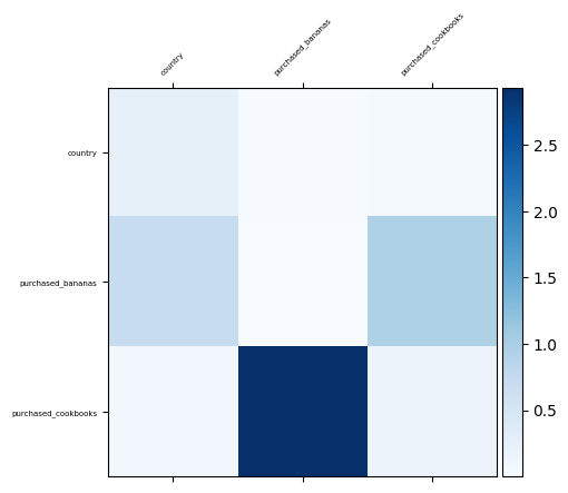
Visualizing feature interactions

Since we already know which feature crosses are important in our data, it would be interesting to verify whether our model has indeed learned these key feature interactions. This can be done by visualizing the learned weight matrix in the cross network, where the weight Wij represents the learned importance of the interaction between features xi and xj.

visualize_layer(
    matrix=cross_network.weights[0].numpy(),
    features=["country", "purchased_bananas", "purchased_cookbooks"],
)

/var/tmp/ipykernel_674880/2224087162.py:11: UserWarning: set_ticklabels() should only be used with a fixed number of ticks, i.e. after set_ticks() or using a FixedLocator.
  ax.set_xticklabels([""] + features, rotation=45, fontsize=10)
/var/tmp/ipykernel_674880/2224087162.py:12: UserWarning: set_ticklabels() should only be used with a fixed number of ticks, i.e. after set_ticks() or using a FixedLocator.
  ax.set_yticklabels([""] + features, fontsize=10)

<Figure size 900x900 with 0 Axes>

png

Real-world example

Let's use the MovieLens 100K dataset. This dataset is used to train models to predict users' movie ratings, based on user-related features and movie-related features.

Preparing the dataset

The dataset processing steps here are similar to what's given in the basic ranking tutorial. Let's load the dataset, and keep only the useful columns.

ratings_ds = tfds.load("movielens/100k-ratings", split="train")
ratings_ds = ratings_ds.map(
    lambda x: (
        {
            "movie_id": int(x["movie_id"]),
            "user_id": int(x["user_id"]),
            "user_gender": int(x["user_gender"]),
            "user_zip_code": x["user_zip_code"],
            "user_occupation_text": x["user_occupation_text"],
            "bucketized_user_age": int(x["bucketized_user_age"]),
        },
        x["user_rating"],  # label
    )
)

For every feature, let's get the list of unique values, i.e., vocabulary, so that we can use that for the embedding layer.

vocabularies = {}
for feature_name in MOVIELENS_CONFIG["int_features"] + MOVIELENS_CONFIG["str_features"]:
    vocabulary = ratings_ds.batch(10_000).map(lambda x, y: x[feature_name])
    vocabularies[feature_name] = np.unique(np.concatenate(list(vocabulary)))

One thing we need to do is to use keras.layers.StringLookup and keras.layers.IntegerLookup to convert all features into indices, which can then be fed into embedding layers.

lookup_layers = {}
lookup_layers.update(
    {
        feature: keras.layers.IntegerLookup(vocabulary=vocabularies[feature])
        for feature in MOVIELENS_CONFIG["int_features"]
    }
)
lookup_layers.update(
    {
        feature: keras.layers.StringLookup(vocabulary=vocabularies[feature])
        for feature in MOVIELENS_CONFIG["str_features"]
    }
)

ratings_ds = ratings_ds.map(
    lambda x, y: (
        {
            feature_name: lookup_layers[feature_name](x[feature_name])
            for feature_name in vocabularies
        },
        y,
    )
)

Let's split our data into train and test sets. We also use cache() and prefetch() for better performance.

ratings_ds = ratings_ds.shuffle(100_000)

train_ds = (
    ratings_ds.take(80_000)
    .batch(MOVIELENS_CONFIG["batch_size"])
    .cache()
    .prefetch(tf.data.AUTOTUNE)
)
test_ds = (
    ratings_ds.skip(80_000)
    .batch(MOVIELENS_CONFIG["batch_size"])
    .take(20_000)
    .cache()
    .prefetch(tf.data.AUTOTUNE)
)

Building the model

The model will have embedding layers, followed by cross and/or feedforward layers.

def get_model(
    dense_num_units_lst,
    embedding_dim=MOVIELENS_CONFIG["embedding_dim"],
    use_cross_layer=False,
    projection_dim=None,
):
    inputs = {}
    embeddings = []
    for feature_name, vocabulary in vocabularies.items():
        inputs[feature_name] = keras.Input(shape=(), dtype="int32", name=feature_name)
        embedding_layer = keras.layers.Embedding(
            input_dim=len(vocabulary) + 1,
            output_dim=embedding_dim,
        )
        embedding = embedding_layer(inputs[feature_name])
        embeddings.append(embedding)

    x = keras.ops.concatenate(embeddings, axis=1)

    # Cross layer.
    if use_cross_layer:
        x = keras_rs.layers.FeatureCross(projection_dim=projection_dim)(x)

    # Dense layer.
    for num_units in dense_num_units_lst:
        x = keras.layers.Dense(num_units, activation="relu")(x)

    x = keras.layers.Dense(1)(x)

    return keras.Model(inputs=inputs, outputs=x)

We have three models - a deep cross network, an optimised deep cross network with a low-rank matrix (to reduce training and serving costs) and a normal deep network without cross layers. The deep cross network is a stacked DCN model, i.e., the inputs are fed to cross layers, followed by feedforward layers. Let's run each model 10 times, and report the average/standard deviation of the RMSE.

cross_network_rmse_list = []
opt_cross_network_rmse_list = []
deep_network_rmse_list = []

for _ in range(10):
    cross_network = get_model(
        dense_num_units_lst=MOVIELENS_CONFIG["dcn_num_units"],
        embedding_dim=MOVIELENS_CONFIG["embedding_dim"],
        use_cross_layer=True,
    )
    rmse, cross_network_num_params = train_and_evaluate(
        learning_rate=MOVIELENS_CONFIG["learning_rate"],
        epochs=MOVIELENS_CONFIG["num_epochs"],
        train_data=train_ds,
        test_data=test_ds,
        model=cross_network,
    )
    cross_network_rmse_list.append(rmse)

    opt_cross_network = get_model(
        dense_num_units_lst=MOVIELENS_CONFIG["dcn_num_units"],
        embedding_dim=MOVIELENS_CONFIG["embedding_dim"],
        use_cross_layer=True,
        projection_dim=MOVIELENS_CONFIG["projection_dim"],
    )
    rmse, opt_cross_network_num_params = train_and_evaluate(
        learning_rate=MOVIELENS_CONFIG["learning_rate"],
        epochs=MOVIELENS_CONFIG["num_epochs"],
        train_data=train_ds,
        test_data=test_ds,
        model=opt_cross_network,
    )
    opt_cross_network_rmse_list.append(rmse)

    deep_network = get_model(dense_num_units_lst=MOVIELENS_CONFIG["deep_net_num_units"])
    rmse, deep_network_num_params = train_and_evaluate(
        learning_rate=MOVIELENS_CONFIG["learning_rate"],
        epochs=MOVIELENS_CONFIG["num_epochs"],
        train_data=train_ds,
        test_data=test_ds,
        model=deep_network,
    )
    deep_network_rmse_list.append(rmse)

print_stats(
    rmse_list=cross_network_rmse_list,
    num_params=cross_network_num_params,
    model_name="Cross Network",
)
print_stats(
    rmse_list=opt_cross_network_rmse_list,
    num_params=opt_cross_network_num_params,
    model_name="Optimised Cross Network",
)
print_stats(
    rmse_list=deep_network_rmse_list,
    num_params=deep_network_num_params,
    model_name="Deep Network",
)

Cross Network: RMSE = 0.8887265503406525 ± 0.02188869864935667; #params = 221953
Optimised Cross Network: RMSE = 0.9222802877426147 ± 0.044382040717192484; #params = 192769
Deep Network: RMSE = 0.8751056969165802 ± 0.029525712693164348; #params = 221953

DCN outperforms a similarly sized DNN with ReLU layers, demonstrating superior performance. Furthermore, the low-rank DCN effectively reduces the number of parameters without compromising accuracy.

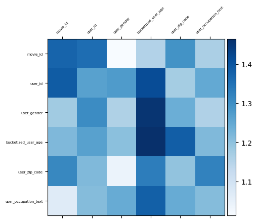
Visualizing feature interactions

Like we did for the toy example, we will plot the weight matrix of the cross layer to see which feature crosses are important. In the previous example, the importance of interactions between the i-th and j-th features is captured by the (i, j)-{th} element of the weight matrix.

In this case, the feature embeddings are of size 32 rather than 1. Therefore, the importance of feature interactions is represented by the (i, j)-th block of the weight matrix, which has dimensions 32 x 32. To quantify the significance of these interactions, we use the Frobenius norm of each block. A larger value implies higher importance.

features = list(vocabularies.keys())
mat = cross_network.weights[len(features)].numpy()
embedding_dim = MOVIELENS_CONFIG["embedding_dim"]

block_norm = np.zeros([len(features), len(features)])

# Compute the norms of the blocks.
for i in range(len(features)):
    for j in range(len(features)):
        block = mat[
            i * embedding_dim : (i + 1) * embedding_dim,
            j * embedding_dim : (j + 1) * embedding_dim,
        ]
        block_norm[i, j] = np.linalg.norm(block, ord="fro")

visualize_layer(
    matrix=block_norm,
    features=features,
)

/var/tmp/ipykernel_674880/2224087162.py:11: UserWarning: set_ticklabels() should only be used with a fixed number of ticks, i.e. after set_ticks() or using a FixedLocator.
  ax.set_xticklabels([""] + features, rotation=45, fontsize=10)
/var/tmp/ipykernel_674880/2224087162.py:12: UserWarning: set_ticklabels() should only be used with a fixed number of ticks, i.e. after set_ticks() or using a FixedLocator.
  ax.set_yticklabels([""] + features, fontsize=10)

<Figure size 900x900 with 0 Axes>

png

And we are all done!

Ranking with Deep and Cross Networks

Introduction

Toy Example

Preparing the dataset

Building the model

Model training

Visualizing feature interactions

Real-world example

Preparing the dataset

Building the model

Visualizing feature interactions