Training & evaluation with the built-in methods
Author: fchollet
Date created: 2019/03/01
Last modified: 2023/06/25
Description: Complete guide to training & evaluation with fit() and evaluate().

Setup
# We import torch & TF so as to use torch Dataloaders & tf.data.Datasets.
import torch
import tensorflow as tf

import os
import numpy as np
import keras
from keras import layers
from keras import ops
Introduction
This guide covers training, evaluation, and prediction (inference) models
when using built-in APIs for training & validation (such as Model.fit(),
Model.evaluate() and Model.predict()).
If you are interested in leveraging fit() while specifying your
own training step function, see the guides on customizing what happens in fit():
- Writing a custom train step with TensorFlow
- Writing a custom train step with JAX
- Writing a custom train step with PyTorch
If you are interested in writing your own training & evaluation loops from scratch, see the guides on writing training loops:
- Writing a training loop with TensorFlow
- Writing a training loop with JAX
- Writing a training loop with PyTorch
In general, whether you are using built-in loops or writing your own, model training & evaluation works strictly in the same way across every kind of Keras model – Sequential models, models built with the Functional API, and models written from scratch via model subclassing.
API overview: a first end-to-end example
When passing data to the built-in training loops of a model, you should either use:
- NumPy arrays (if your data is small and fits in memory)
- Subclasses of
keras.utils.PyDataset tf.data.Datasetobjects- PyTorch
DataLoaderinstances
In the next few paragraphs, we'll use the MNIST dataset as NumPy arrays, in order to demonstrate how to use optimizers, losses, and metrics. Afterwards, we'll take a close look at each of the other options.
Let's consider the following model (here, we build in with the Functional API, but it could be a Sequential model or a subclassed model as well):
inputs = keras.Input(shape=(784,), name="digits")
x = layers.Dense(64, activation="relu", name="dense_1")(inputs)
x = layers.Dense(64, activation="relu", name="dense_2")(x)
outputs = layers.Dense(10, activation="softmax", name="predictions")(x)

model = keras.Model(inputs=inputs, outputs=outputs)
Here's what the typical end-to-end workflow looks like, consisting of:
- Training
- Validation on a holdout set generated from the original training data
- Evaluation on the test data
We'll use MNIST data for this example.
(x_train, y_train), (x_test, y_test) = keras.datasets.mnist.load_data()

# Preprocess the data (these are NumPy arrays)
x_train = x_train.reshape(60000, 784).astype("float32") / 255
x_test = x_test.reshape(10000, 784).astype("float32") / 255

y_train = y_train.astype("float32")
y_test = y_test.astype("float32")

# Reserve 10,000 samples for validation
x_val = x_train[-10000:]
y_val = y_train[-10000:]
x_train = x_train[:-10000]
y_train = y_train[:-10000]
We specify the training configuration (optimizer, loss, metrics):
model.compile(
    optimizer=keras.optimizers.RMSprop(),  # Optimizer
    # Loss function to minimize
    loss=keras.losses.SparseCategoricalCrossentropy(),
    # List of metrics to monitor
    metrics=[keras.metrics.SparseCategoricalAccuracy()],
)
We call fit(), which will train the model by slicing the data into "batches" of size
batch_size, and repeatedly iterating over the entire dataset for a given number of
epochs.
print("Fit model on training data")
history = model.fit(
    x_train,
    y_train,
    batch_size=64,
    epochs=2,
    # We pass some validation for
    # monitoring validation loss and metrics
    # at the end of each epoch
    validation_data=(x_val, y_val),
)
Fit model on training data
Epoch 1/2
 782/782 ━━━━━━━━━━━━━━━━━━━━ 1s 955us/step - loss: 0.5740 - sparse_categorical_accuracy: 0.8368 - val_loss: 0.2040 - val_sparse_categorical_accuracy: 0.9420
Epoch 2/2
 782/782 ━━━━━━━━━━━━━━━━━━━━ 0s 390us/step - loss: 0.1745 - sparse_categorical_accuracy: 0.9492 - val_loss: 0.1415 - val_sparse_categorical_accuracy: 0.9581
The returned history object holds a record of the loss values and metric values
during training:
print(history.history)
{'loss': [0.34448376297950745, 0.16419583559036255], 'sparse_categorical_accuracy': [0.9008600115776062, 0.9509199857711792], 'val_loss': [0.20404714345932007, 0.14145156741142273], 'val_sparse_categorical_accuracy': [0.9419999718666077, 0.9581000208854675]}
We evaluate the model on the test data via evaluate():
# Evaluate the model on the test data using `evaluate`
print("Evaluate on test data")
results = model.evaluate(x_test, y_test, batch_size=128)
print("test loss, test acc:", results)

# Generate predictions (probabilities -- the output of the last layer)
# on new data using `predict`
print("Generate predictions for 3 samples")
predictions = model.predict(x_test[:3])
print("predictions shape:", predictions.shape)
Evaluate on test data
 79/79 ━━━━━━━━━━━━━━━━━━━━ 0s 271us/step - loss: 0.1670 - sparse_categorical_accuracy: 0.9489
test loss, test acc: [0.1484374850988388, 0.9550999999046326]
Generate predictions for 3 samples
 1/1 ━━━━━━━━━━━━━━━━━━━━ 0s 33ms/step
predictions shape: (3, 10)
Now, let's review each piece of this workflow in detail.
The compile() method: specifying a loss, metrics, and an optimizer
To train a model with fit(), you need to specify a loss function, an optimizer, and
optionally, some metrics to monitor.
You pass these to the model as arguments to the compile() method:
model.compile(
    optimizer=keras.optimizers.RMSprop(learning_rate=1e-3),
    loss=keras.losses.SparseCategoricalCrossentropy(),
    metrics=[keras.metrics.SparseCategoricalAccuracy()],
)
The metrics argument should be a list – your model can have any number of metrics.
If your model has multiple outputs, you can specify different losses and metrics for each output, and you can modulate the contribution of each output to the total loss of the model. You will find more details about this in the Passing data to multi-input, multi-output models section.
Note that if you're satisfied with the default settings, in many cases the optimizer, loss, and metrics can be specified via string identifiers as a shortcut:
model.compile(
    optimizer="rmsprop",
    loss="sparse_categorical_crossentropy",
    metrics=["sparse_categorical_accuracy"],
)
For later reuse, let's put our model definition and compile step in functions; we will call them several times across different examples in this guide.
def get_uncompiled_model():
    inputs = keras.Input(shape=(784,), name="digits")
    x = layers.Dense(64, activation="relu", name="dense_1")(inputs)
    x = layers.Dense(64, activation="relu", name="dense_2")(x)
    outputs = layers.Dense(10, activation="softmax", name="predictions")(x)
    model = keras.Model(inputs=inputs, outputs=outputs)
    return model


def get_compiled_model():
    model = get_uncompiled_model()
    model.compile(
        optimizer="rmsprop",
        loss="sparse_categorical_crossentropy",
        metrics=["sparse_categorical_accuracy"],
    )
    return model
Many built-in optimizers, losses, and metrics are available
In general, you won't have to create your own losses, metrics, or optimizers from scratch, because what you need is likely to be already part of the Keras API:
Optimizers:
SGD()(with or without momentum)RMSprop()Adam()- etc.
Losses:
MeanSquaredError()KLDivergence()CosineSimilarity()- etc.
Metrics:
AUC()Precision()Recall()- etc.
Custom losses
If you need to create a custom loss, Keras provides three ways to do so.
The first method involves creating a function that accepts inputs y_true and
y_pred. The following example shows a loss function that computes the mean squared
error between the real data and the predictions:
def custom_mean_squared_error(y_true, y_pred):
    return ops.mean(ops.square(y_true - y_pred), axis=-1)


model = get_uncompiled_model()
model.compile(optimizer=keras.optimizers.Adam(), loss=custom_mean_squared_error)

# We need to one-hot encode the labels to use MSE
y_train_one_hot = ops.one_hot(y_train, num_classes=10)
model.fit(x_train, y_train_one_hot, batch_size=64, epochs=1)
 782/782 ━━━━━━━━━━━━━━━━━━━━ 1s 525us/step - loss: 0.0277

<keras.src.callbacks.history.History at 0x2e5dde350>
If you need a loss function that takes in parameters beside y_true and y_pred, you
can subclass the keras.losses.Loss class and implement the following two methods:
__init__(self): accept parameters to pass during the call of your loss functioncall(self, y_true, y_pred): use the targets (y_true) and the model predictions (y_pred) to compute the model's loss
Let's say you want to use mean squared error, but with an added term that will de-incentivize prediction values far from 0.5 (we assume that the categorical targets are one-hot encoded and take values between 0 and 1). This creates an incentive for the model not to be too confident, which may help reduce overfitting (we won't know if it works until we try!).
Here's how you would do it:
class CustomMSE(keras.losses.Loss):
    def __init__(self, regularization_factor=0.1, name="custom_mse"):
        super().__init__(name=name)
        self.regularization_factor = regularization_factor

    def call(self, y_true, y_pred):
        mse = ops.mean(ops.square(y_true - y_pred), axis=-1)
        reg = ops.mean(ops.square(0.5 - y_pred), axis=-1)
        return mse + reg * self.regularization_factor


model = get_uncompiled_model()
model.compile(optimizer=keras.optimizers.Adam(), loss=CustomMSE())

y_train_one_hot = ops.one_hot(y_train, num_classes=10)
model.fit(x_train, y_train_one_hot, batch_size=64, epochs=1)
 782/782 ━━━━━━━━━━━━━━━━━━━━ 1s 532us/step - loss: 0.0492

<keras.src.callbacks.history.History at 0x2e5d0d360>
Custom metrics
If you need a metric that isn't part of the API, you can easily create custom metrics
by subclassing the keras.metrics.Metric class. You will need to implement 4
methods:
__init__(self), in which you will create state variables for your metric.update_state(self, y_true, y_pred, sample_weight=None), which uses the targets y_true and the model predictions y_pred to update the state variables.result(self), which uses the state variables to compute the final results.reset_state(self), which reinitializes the state of the metric.
State update and results computation are kept separate (in update_state() and
result(), respectively) because in some cases, the results computation might be very
expensive and would only be done periodically.
Here's a simple example showing how to implement a CategoricalTruePositives metric
that counts how many samples were correctly classified as belonging to a given class:
class CategoricalTruePositives(keras.metrics.Metric):
    def __init__(self, name="categorical_true_positives", **kwargs):
        super().__init__(name=name, **kwargs)
        self.true_positives = self.add_variable(
            shape=(), name="ctp", initializer="zeros"
        )

    def update_state(self, y_true, y_pred, sample_weight=None):
        y_pred = ops.reshape(ops.argmax(y_pred, axis=1), (-1, 1))
        values = ops.cast(y_true, "int32") == ops.cast(y_pred, "int32")
        values = ops.cast(values, "float32")
        if sample_weight is not None:
            sample_weight = ops.cast(sample_weight, "float32")
            values = ops.multiply(values, sample_weight)
        self.true_positives.assign_add(ops.sum(values))

    def result(self):
        return self.true_positives.value

    def reset_state(self):
        # The state of the metric will be reset at the start of each epoch.
        self.true_positives.assign(0.0)


model = get_uncompiled_model()
model.compile(
    optimizer=keras.optimizers.RMSprop(learning_rate=1e-3),
    loss=keras.losses.SparseCategoricalCrossentropy(),
    metrics=[CategoricalTruePositives()],
)
model.fit(x_train, y_train, batch_size=64, epochs=3)
Epoch 1/3
 782/782 ━━━━━━━━━━━━━━━━━━━━ 1s 568us/step - categorical_true_positives: 180967.9219 - loss: 0.5876
Epoch 2/3
 782/782 ━━━━━━━━━━━━━━━━━━━━ 0s 377us/step - categorical_true_positives: 182141.9375 - loss: 0.1733
Epoch 3/3
 782/782 ━━━━━━━━━━━━━━━━━━━━ 0s 377us/step - categorical_true_positives: 182303.5312 - loss: 0.1180

<keras.src.callbacks.history.History at 0x2e5f02d10>
Handling losses and metrics that don't fit the standard signature
The overwhelming majority of losses and metrics can be computed from y_true and
y_pred, where y_pred is an output of your model – but not all of them. For
instance, a regularization loss may only require the activation of a layer (there are
no targets in this case), and this activation may not be a model output.
In such cases, you can call self.add_loss(loss_value) from inside the call method of
a custom layer. Losses added in this way get added to the "main" loss during training
(the one passed to compile()). Here's a simple example that adds activity
regularization (note that activity regularization is built-in in all Keras layers –
this layer is just for the sake of providing a concrete example):
class ActivityRegularizationLayer(layers.Layer):
    def call(self, inputs):
        self.add_loss(ops.sum(inputs) * 0.1)
        return inputs  # Pass-through layer.


inputs = keras.Input(shape=(784,), name="digits")
x = layers.Dense(64, activation="relu", name="dense_1")(inputs)

# Insert activity regularization as a layer
x = ActivityRegularizationLayer()(x)

x = layers.Dense(64, activation="relu", name="dense_2")(x)
outputs = layers.Dense(10, name="predictions")(x)

model = keras.Model(inputs=inputs, outputs=outputs)
model.compile(
    optimizer=keras.optimizers.RMSprop(learning_rate=1e-3),
    loss=keras.losses.SparseCategoricalCrossentropy(from_logits=True),
)

# The displayed loss will be much higher than before
# due to the regularization component.
model.fit(x_train, y_train, batch_size=64, epochs=1)
 782/782 ━━━━━━━━━━━━━━━━━━━━ 1s 505us/step - loss: 3.4083

<keras.src.callbacks.history.History at 0x2e60226b0>
Note that when you pass losses via add_loss(), it becomes possible to call
compile() without a loss function, since the model already has a loss to minimize.
Consider the following LogisticEndpoint layer: it takes as inputs
targets & logits, and it tracks a crossentropy loss via add_loss().
class LogisticEndpoint(keras.layers.Layer):
    def __init__(self, name=None):
        super().__init__(name=name)
        self.loss_fn = keras.losses.BinaryCrossentropy(from_logits=True)

    def call(self, targets, logits, sample_weights=None):
        # Compute the training-time loss value and add it
        # to the layer using `self.add_loss()`.
        loss = self.loss_fn(targets, logits, sample_weights)
        self.add_loss(loss)

        # Return the inference-time prediction tensor (for `.predict()`).
        return ops.softmax(logits)
You can use it in a model with two inputs (input data & targets), compiled without a
loss argument, like this:
inputs = keras.Input(shape=(3,), name="inputs")
targets = keras.Input(shape=(10,), name="targets")
logits = keras.layers.Dense(10)(inputs)
predictions = LogisticEndpoint(name="predictions")(targets, logits)

model = keras.Model(inputs=[inputs, targets], outputs=predictions)
model.compile(optimizer="adam")  # No loss argument!

data = {
    "inputs": np.random.random((3, 3)),
    "targets": np.random.random((3, 10)),
}
model.fit(data)
 1/1 ━━━━━━━━━━━━━━━━━━━━ 0s 89ms/step - loss: 0.6982

<keras.src.callbacks.history.History at 0x2e5cc91e0>
For more information about training multi-input models, see the section Passing data to multi-input, multi-output models.
Automatically setting apart a validation holdout set
In the first end-to-end example you saw, we used the validation_data argument to pass
a tuple of NumPy arrays (x_val, y_val) to the model for evaluating a validation loss
and validation metrics at the end of each epoch.
Here's another option: the argument validation_split allows you to automatically
reserve part of your training data for validation. The argument value represents the
fraction of the data to be reserved for validation, so it should be set to a number
higher than 0 and lower than 1. For instance, validation_split=0.2 means "use 20% of
the data for validation", and validation_split=0.6 means "use 60% of the data for
validation".
The way the validation is computed is by taking the last x% samples of the arrays
received by the fit() call, before any shuffling.
Note that you can only use validation_split when training with NumPy data.
model = get_compiled_model()
model.fit(x_train, y_train, batch_size=64, validation_split=0.2, epochs=1)
 625/625 ━━━━━━━━━━━━━━━━━━━━ 1s 563us/step - loss: 0.6161 - sparse_categorical_accuracy: 0.8259 - val_loss: 0.2379 - val_sparse_categorical_accuracy: 0.9302

<keras.src.callbacks.history.History at 0x2e6007610>
Training & evaluation using tf.data Datasets
In the past few paragraphs, you've seen how to handle losses, metrics, and optimizers,
and you've seen how to use the validation_data and validation_split arguments in
fit(), when your data is passed as NumPy arrays.
Another option is to use an iterator-like, such as a tf.data.Dataset, a
PyTorch DataLoader, or a Keras PyDataset. Let's take look at the former.
The tf.data API is a set of utilities in TensorFlow 2.0 for loading and preprocessing
data in a way that's fast and scalable. For a complete guide about creating Datasets,
see the tf.data documentation.
You can use tf.data to train your Keras
models regardless of the backend you're using –
whether it's JAX, PyTorch, or TensorFlow.
You can pass a Dataset instance directly to the methods fit(), evaluate(), and
predict():
model = get_compiled_model()

# First, let's create a training Dataset instance.
# For the sake of our example, we'll use the same MNIST data as before.
train_dataset = tf.data.Dataset.from_tensor_slices((x_train, y_train))
# Shuffle and slice the dataset.
train_dataset = train_dataset.shuffle(buffer_size=1024).batch(64)

# Now we get a test dataset.
test_dataset = tf.data.Dataset.from_tensor_slices((x_test, y_test))
test_dataset = test_dataset.batch(64)

# Since the dataset already takes care of batching,
# we don't pass a `batch_size` argument.
model.fit(train_dataset, epochs=3)

# You can also evaluate or predict on a dataset.
print("Evaluate")
result = model.evaluate(test_dataset)
dict(zip(model.metrics_names, result))
Epoch 1/3
 782/782 ━━━━━━━━━━━━━━━━━━━━ 1s 688us/step - loss: 0.5631 - sparse_categorical_accuracy: 0.8458
Epoch 2/3
 782/782 ━━━━━━━━━━━━━━━━━━━━ 0s 512us/step - loss: 0.1703 - sparse_categorical_accuracy: 0.9484
Epoch 3/3
 782/782 ━━━━━━━━━━━━━━━━━━━━ 0s 506us/step - loss: 0.1187 - sparse_categorical_accuracy: 0.9640
Evaluate
 157/157 ━━━━━━━━━━━━━━━━━━━━ 0s 622us/step - loss: 0.1380 - sparse_categorical_accuracy: 0.9582

{'loss': 0.11913617700338364, 'compile_metrics': 0.965399980545044}
Note that the Dataset is reset at the end of each epoch, so it can be reused of the next epoch.
If you want to run training only on a specific number of batches from this Dataset, you
can pass the steps_per_epoch argument, which specifies how many training steps the
model should run using this Dataset before moving on to the next epoch.
model = get_compiled_model()

# Prepare the training dataset
train_dataset = tf.data.Dataset.from_tensor_slices((x_train, y_train))
train_dataset = train_dataset.shuffle(buffer_size=1024).batch(64)

# Only use the 100 batches per epoch (that's 64 * 100 samples)
model.fit(train_dataset, epochs=3, steps_per_epoch=100)
Epoch 1/3
 100/100 ━━━━━━━━━━━━━━━━━━━━ 0s 508us/step - loss: 1.2000 - sparse_categorical_accuracy: 0.6822
Epoch 2/3
 100/100 ━━━━━━━━━━━━━━━━━━━━ 0s 481us/step - loss: 0.4004 - sparse_categorical_accuracy: 0.8827
Epoch 3/3
 100/100 ━━━━━━━━━━━━━━━━━━━━ 0s 471us/step - loss: 0.3546 - sparse_categorical_accuracy: 0.8968

<keras.src.callbacks.history.History at 0x2e64df400>
You can also pass a Dataset instance as the validation_data argument in fit():
model = get_compiled_model()

# Prepare the training dataset
train_dataset = tf.data.Dataset.from_tensor_slices((x_train, y_train))
train_dataset = train_dataset.shuffle(buffer_size=1024).batch(64)

# Prepare the validation dataset
val_dataset = tf.data.Dataset.from_tensor_slices((x_val, y_val))
val_dataset = val_dataset.batch(64)

model.fit(train_dataset, epochs=1, validation_data=val_dataset)
 782/782 ━━━━━━━━━━━━━━━━━━━━ 1s 837us/step - loss: 0.5569 - sparse_categorical_accuracy: 0.8508 - val_loss: 0.1711 - val_sparse_categorical_accuracy: 0.9527

<keras.src.callbacks.history.History at 0x2e641e920>
At the end of each epoch, the model will iterate over the validation dataset and compute the validation loss and validation metrics.
If you want to run validation only on a specific number of batches from this dataset,
you can pass the validation_steps argument, which specifies how many validation
steps the model should run with the validation dataset before interrupting validation
and moving on to the next epoch:
model = get_compiled_model()

# Prepare the training dataset
train_dataset = tf.data.Dataset.from_tensor_slices((x_train, y_train))
train_dataset = train_dataset.shuffle(buffer_size=1024).batch(64)

# Prepare the validation dataset
val_dataset = tf.data.Dataset.from_tensor_slices((x_val, y_val))
val_dataset = val_dataset.batch(64)

model.fit(
    train_dataset,
    epochs=1,
    # Only run validation using the first 10 batches of the dataset
    # using the `validation_steps` argument
    validation_data=val_dataset,
    validation_steps=10,
)
 782/782 ━━━━━━━━━━━━━━━━━━━━ 1s 771us/step - loss: 0.5562 - sparse_categorical_accuracy: 0.8436 - val_loss: 0.3345 - val_sparse_categorical_accuracy: 0.9062

<keras.src.callbacks.history.History at 0x2f9542e00>
Note that the validation dataset will be reset after each use (so that you will always be evaluating on the same samples from epoch to epoch).
The argument validation_split (generating a holdout set from the training data) is
not supported when training from Dataset objects, since this feature requires the
ability to index the samples of the datasets, which is not possible in general with
the Dataset API.
Training & evaluation using PyDataset instances
keras.utils.PyDataset is a utility that you can subclass to obtain
a Python generator with two important properties:
- It works well with multiprocessing.
- It can be shuffled (e.g. when passing
shuffle=Trueinfit()).
A PyDataset must implement two methods:
__getitem____len__
The method __getitem__ should return a complete batch.
If you want to modify your dataset between epochs, you may implement on_epoch_end.
Here's a quick example:
class ExamplePyDataset(keras.utils.PyDataset):
    def __init__(self, x, y, batch_size, **kwargs):
        super().__init__(**kwargs)
        self.x = x
        self.y = y
        self.batch_size = batch_size

    def __len__(self):
        return int(np.ceil(len(self.x) / float(self.batch_size)))

    def __getitem__(self, idx):
        batch_x = self.x[idx * self.batch_size : (idx + 1) * self.batch_size]
        batch_y = self.y[idx * self.batch_size : (idx + 1) * self.batch_size]
        return batch_x, batch_y


train_py_dataset = ExamplePyDataset(x_train, y_train, batch_size=32)
val_py_dataset = ExamplePyDataset(x_val, y_val, batch_size=32)
To fit the model, pass the dataset instead as the x argument (no need for a y
argument since the dataset includes the targets), and pass the validation dataset
as the validation_data argument. And no need for the batch_size argument, since
the dataset is already batched!
model = get_compiled_model()
model.fit(train_py_dataset, batch_size=64, validation_data=val_py_dataset, epochs=1)
 1563/1563 ━━━━━━━━━━━━━━━━━━━━ 1s 443us/step - loss: 0.5217 - sparse_categorical_accuracy: 0.8473 - val_loss: 0.1576 - val_sparse_categorical_accuracy: 0.9525

<keras.src.callbacks.history.History at 0x2f9c8d120>
Evaluating the model is just as easy:
model.evaluate(val_py_dataset)
 313/313 ━━━━━━━━━━━━━━━━━━━━ 0s 157us/step - loss: 0.1821 - sparse_categorical_accuracy: 0.9450

[0.15764616429805756, 0.9524999856948853]
Importantly, PyDataset objects support three common constructor arguments
that handle the parallel processing configuration:
workers: Number of workers to use in multithreading or multiprocessing. Typically, you'd set it to the number of cores on your CPU.use_multiprocessing: Whether to use Python multiprocessing for parallelism. Setting this toTruemeans that your dataset will be replicated in multiple forked processes. This is necessary to gain compute-level (rather than I/O level) benefits from parallelism. However it can only be set toTrueif your dataset can be safely pickled.max_queue_size: Maximum number of batches to keep in the queue when iterating over the dataset in a multithreaded or multipricessed setting. You can reduce this value to reduce the CPU memory consumption of your dataset. It defaults to 10.
By default, multiprocessing is disabled (use_multiprocessing=False) and only
one thread is used. You should make sure to only turn on use_multiprocessing if
your code is running inside a Python if __name__ == "__main__": block in order
to avoid issues.
Here's a 4-thread, non-multiprocessed example:
train_py_dataset = ExamplePyDataset(x_train, y_train, batch_size=32, workers=4)
val_py_dataset = ExamplePyDataset(x_val, y_val, batch_size=32, workers=4)

model = get_compiled_model()
model.fit(train_py_dataset, batch_size=64, validation_data=val_py_dataset, epochs=1)
 1563/1563 ━━━━━━━━━━━━━━━━━━━━ 1s 561us/step - loss: 0.5146 - sparse_categorical_accuracy: 0.8516 - val_loss: 0.1623 - val_sparse_categorical_accuracy: 0.9514

<keras.src.callbacks.history.History at 0x2e7fd5ea0>
Training & evaluation using PyTorch DataLoader objects
All built-in training and evaluation APIs are also compatible with torch.utils.data.Dataset and
torch.utils.data.DataLoader objects – regardless of whether you're using the PyTorch backend,
or the JAX or TensorFlow backends. Let's take a look at a simple example.
Unlike PyDataset which are batch-centric, PyTorch Dataset objects are sample-centric:
the __len__ method returns the number of samples,
and the __getitem__ method returns a specific sample.
class ExampleTorchDataset(torch.utils.data.Dataset):
    def __init__(self, x, y):
        self.x = x
        self.y = y

    def __len__(self):
        return len(self.x)

    def __getitem__(self, idx):
        return self.x[idx], self.y[idx]


train_torch_dataset = ExampleTorchDataset(x_train, y_train)
val_torch_dataset = ExampleTorchDataset(x_val, y_val)
To use a PyTorch Dataset, you need to wrap it into a Dataloader which takes care
of batching and shuffling:
train_dataloader = torch.utils.data.DataLoader(
    train_torch_dataset, batch_size=32, shuffle=True
)
val_dataloader = torch.utils.data.DataLoader(
    val_torch_dataset, batch_size=32, shuffle=True
)
Now you can use them in the Keras API just like any other iterator:
model = get_compiled_model()
model.fit(train_dataloader, batch_size=64, validation_data=val_dataloader, epochs=1)
model.evaluate(val_dataloader)
 1563/1563 ━━━━━━━━━━━━━━━━━━━━ 1s 575us/step - loss: 0.5051 - sparse_categorical_accuracy: 0.8568 - val_loss: 0.1613 - val_sparse_categorical_accuracy: 0.9528
 313/313 ━━━━━━━━━━━━━━━━━━━━ 0s 278us/step - loss: 0.1551 - sparse_categorical_accuracy: 0.9541

[0.16209803521633148, 0.9527999758720398]
Using sample weighting and class weighting
With the default settings the weight of a sample is decided by its frequency in the dataset. There are two methods to weight the data, independent of sample frequency:
- Class weights
- Sample weights
Class weights
This is set by passing a dictionary to the class_weight argument to
Model.fit(). This dictionary maps class indices to the weight that should
be used for samples belonging to this class.
This can be used to balance classes without resampling, or to train a model that gives more importance to a particular class.
For instance, if class "0" is half as represented as class "1" in your data,
you could use Model.fit(..., class_weight={0: 1., 1: 0.5}).
Here's a NumPy example where we use class weights or sample weights to give more importance to the correct classification of class #5 (which is the digit "5" in the MNIST dataset).
class_weight = {
    0: 1.0,
    1: 1.0,
    2: 1.0,
    3: 1.0,
    4: 1.0,
    # Set weight "2" for class "5",
    # making this class 2x more important
    5: 2.0,
    6: 1.0,
    7: 1.0,
    8: 1.0,
    9: 1.0,
}

print("Fit with class weight")
model = get_compiled_model()
model.fit(x_train, y_train, class_weight=class_weight, batch_size=64, epochs=1)
Fit with class weight
 782/782 ━━━━━━━━━━━━━━━━━━━━ 1s 534us/step - loss: 0.6205 - sparse_categorical_accuracy: 0.8375

<keras.src.callbacks.history.History at 0x298d44eb0>
Sample weights
For fine grained control, or if you are not building a classifier, you can use "sample weights".
- When training from NumPy data: Pass the
sample_weightargument toModel.fit(). - When training from
tf.dataor any other sort of iterator: Yield(input_batch, label_batch, sample_weight_batch)tuples.
A "sample weights" array is an array of numbers that specify how much weight each sample in a batch should have in computing the total loss. It is commonly used in imbalanced classification problems (the idea being to give more weight to rarely-seen classes).
When the weights used are ones and zeros, the array can be used as a mask for the loss function (entirely discarding the contribution of certain samples to the total loss).
sample_weight = np.ones(shape=(len(y_train),))
sample_weight[y_train == 5] = 2.0

print("Fit with sample weight")
model = get_compiled_model()
model.fit(x_train, y_train, sample_weight=sample_weight, batch_size=64, epochs=1)
Fit with sample weight
 782/782 ━━━━━━━━━━━━━━━━━━━━ 1s 546us/step - loss: 0.6397 - sparse_categorical_accuracy: 0.8388

<keras.src.callbacks.history.History at 0x298e066e0>
Here's a matching Dataset example:
sample_weight = np.ones(shape=(len(y_train),))
sample_weight[y_train == 5] = 2.0

# Create a Dataset that includes sample weights
# (3rd element in the return tuple).
train_dataset = tf.data.Dataset.from_tensor_slices((x_train, y_train, sample_weight))

# Shuffle and slice the dataset.
train_dataset = train_dataset.shuffle(buffer_size=1024).batch(64)

model = get_compiled_model()
model.fit(train_dataset, epochs=1)
 782/782 ━━━━━━━━━━━━━━━━━━━━ 1s 651us/step - loss: 0.5971 - sparse_categorical_accuracy: 0.8445

<keras.src.callbacks.history.History at 0x312854100>
Passing data to multi-input, multi-output models
In the previous examples, we were considering a model with a single input (a tensor of
shape (764,)) and a single output (a prediction tensor of shape (10,)). But what
about models that have multiple inputs or outputs?
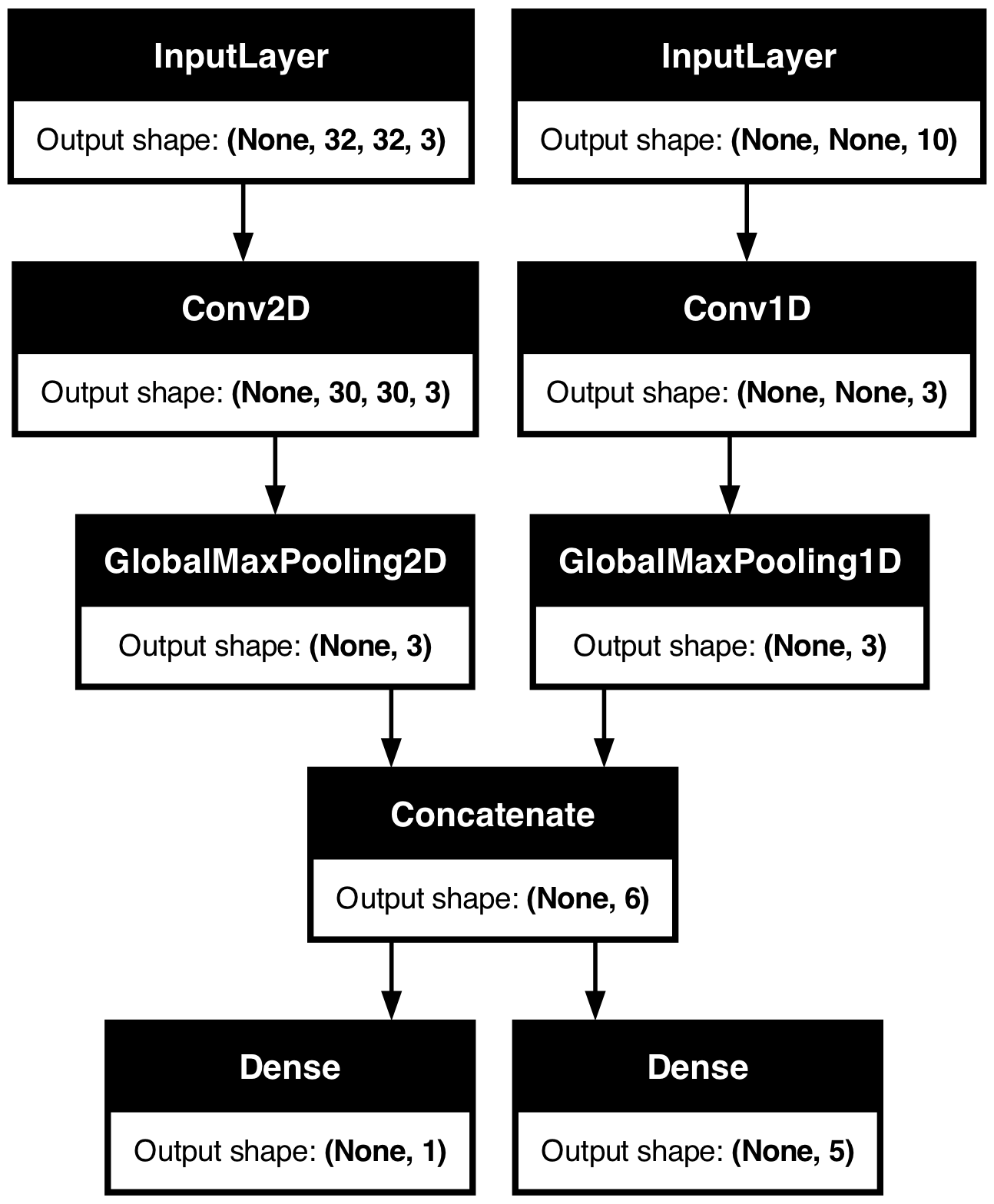
Consider the following model, which has an image input of shape (32, 32, 3) (that's
(height, width, channels)) and a time series input of shape (None, 10) (that's
(timesteps, features)). Our model will have two outputs computed from the
combination of these inputs: a "score" (of shape (1,)) and a probability
distribution over five classes (of shape (5,)).
image_input = keras.Input(shape=(32, 32, 3), name="img_input")
timeseries_input = keras.Input(shape=(None, 10), name="ts_input")

x1 = layers.Conv2D(3, 3)(image_input)
x1 = layers.GlobalMaxPooling2D()(x1)

x2 = layers.Conv1D(3, 3)(timeseries_input)
x2 = layers.GlobalMaxPooling1D()(x2)

x = layers.concatenate([x1, x2])

score_output = layers.Dense(1, name="score_output")(x)
class_output = layers.Dense(5, name="class_output")(x)

model = keras.Model(
    inputs=[image_input, timeseries_input], outputs=[score_output, class_output]
)
Let's plot this model, so you can clearly see what we're doing here (note that the shapes shown in the plot are batch shapes, rather than per-sample shapes).
keras.utils.plot_model(model, "multi_input_and_output_model.png", show_shapes=True)
At compilation time, we can specify different losses to different outputs, by passing the loss functions as a list:
model.compile(
    optimizer=keras.optimizers.RMSprop(1e-3),
    loss=[
        keras.losses.MeanSquaredError(),
        keras.losses.CategoricalCrossentropy(),
    ],
)
If we only passed a single loss function to the model, the same loss function would be applied to every output (which is not appropriate here).
Likewise for metrics:
model.compile(
    optimizer=keras.optimizers.RMSprop(1e-3),
    loss=[
        keras.losses.MeanSquaredError(),
        keras.losses.CategoricalCrossentropy(),
    ],
    metrics=[
        [
            keras.metrics.MeanAbsolutePercentageError(),
            keras.metrics.MeanAbsoluteError(),
        ],
        [keras.metrics.CategoricalAccuracy()],
    ],
)
Since we gave names to our output layers, we could also specify per-output losses and metrics via a dict:
model.compile(
    optimizer=keras.optimizers.RMSprop(1e-3),
    loss={
        "score_output": keras.losses.MeanSquaredError(),
        "class_output": keras.losses.CategoricalCrossentropy(),
    },
    metrics={
        "score_output": [
            keras.metrics.MeanAbsolutePercentageError(),
            keras.metrics.MeanAbsoluteError(),
        ],
        "class_output": [keras.metrics.CategoricalAccuracy()],
    },
)
We recommend the use of explicit names and dicts if you have more than 2 outputs.
It's possible to give different weights to different output-specific losses (for
instance, one might wish to privilege the "score" loss in our example, by giving to 2x
the importance of the class loss), using the loss_weights argument:
model.compile(
    optimizer=keras.optimizers.RMSprop(1e-3),
    loss={
        "score_output": keras.losses.MeanSquaredError(),
        "class_output": keras.losses.CategoricalCrossentropy(),
    },
    metrics={
        "score_output": [
            keras.metrics.MeanAbsolutePercentageError(),
            keras.metrics.MeanAbsoluteError(),
        ],
        "class_output": [keras.metrics.CategoricalAccuracy()],
    },
    loss_weights={"score_output": 2.0, "class_output": 1.0},
)
You could also choose not to compute a loss for certain outputs, if these outputs are meant for prediction but not for training:
# List loss version
model.compile(
    optimizer=keras.optimizers.RMSprop(1e-3),
    loss=[None, keras.losses.CategoricalCrossentropy()],
)

# Or dict loss version
model.compile(
    optimizer=keras.optimizers.RMSprop(1e-3),
    loss={"class_output": keras.losses.CategoricalCrossentropy()},
)
Passing data to a multi-input or multi-output model in fit() works in a similar way as
specifying a loss function in compile: you can pass lists of NumPy arrays (with
1:1 mapping to the outputs that received a loss function) or dicts mapping output
names to NumPy arrays.
model.compile(
    optimizer=keras.optimizers.RMSprop(1e-3),
    loss=[
        keras.losses.MeanSquaredError(),
        keras.losses.CategoricalCrossentropy(),
    ],
)

# Generate dummy NumPy data
img_data = np.random.random_sample(size=(100, 32, 32, 3))
ts_data = np.random.random_sample(size=(100, 20, 10))
score_targets = np.random.random_sample(size=(100, 1))
class_targets = np.random.random_sample(size=(100, 5))

# Fit on lists
model.fit([img_data, ts_data], [score_targets, class_targets], batch_size=32, epochs=1)

# Alternatively, fit on dicts
model.fit(
    {"img_input": img_data, "ts_input": ts_data},
    {"score_output": score_targets, "class_output": class_targets},
    batch_size=32,
    epochs=1,
)
 4/4 ━━━━━━━━━━━━━━━━━━━━ 0s 62ms/step - loss: 18.0146
 4/4 ━━━━━━━━━━━━━━━━━━━━ 0s 56ms/step - loss: 17.6494

<keras.src.callbacks.history.History at 0x31a6c5810>
Here's the Dataset use case: similarly as what we did for NumPy arrays, the Dataset
should return a tuple of dicts.
train_dataset = tf.data.Dataset.from_tensor_slices(
    (
        {"img_input": img_data, "ts_input": ts_data},
        {"score_output": score_targets, "class_output": class_targets},
    )
)
train_dataset = train_dataset.shuffle(buffer_size=1024).batch(64)

model.fit(train_dataset, epochs=1)
 2/2 ━━━━━━━━━━━━━━━━━━━━ 0s 197ms/step - loss: 17.8578

<keras.src.callbacks.history.History at 0x17c7e5690>
Using callbacks
Callbacks in Keras are objects that are called at different points during training (at the start of an epoch, at the end of a batch, at the end of an epoch, etc.). They can be used to implement certain behaviors, such as:
- Doing validation at different points during training (beyond the built-in per-epoch validation)
- Checkpointing the model at regular intervals or when it exceeds a certain accuracy threshold
- Changing the learning rate of the model when training seems to be plateauing
- Doing fine-tuning of the top layers when training seems to be plateauing
- Sending email or instant message notifications when training ends or where a certain performance threshold is exceeded
- Etc.
Callbacks can be passed as a list to your call to fit():
model = get_compiled_model()

callbacks = [
    keras.callbacks.EarlyStopping(
        # Stop training when `val_loss` is no longer improving
        monitor="val_loss",
        # "no longer improving" being defined as "no better than 1e-2 less"
        min_delta=1e-2,
        # "no longer improving" being further defined as "for at least 2 epochs"
        patience=2,
        verbose=1,
    )
]
model.fit(
    x_train,
    y_train,
    epochs=20,
    batch_size=64,
    callbacks=callbacks,
    validation_split=0.2,
)
Epoch 1/20
 625/625 ━━━━━━━━━━━━━━━━━━━━ 1s 622us/step - loss: 0.6245 - sparse_categorical_accuracy: 0.8275 - val_loss: 0.2231 - val_sparse_categorical_accuracy: 0.9330
Epoch 2/20
 625/625 ━━━━━━━━━━━━━━━━━━━━ 0s 404us/step - loss: 0.1809 - sparse_categorical_accuracy: 0.9460 - val_loss: 0.1727 - val_sparse_categorical_accuracy: 0.9476
Epoch 3/20
 625/625 ━━━━━━━━━━━━━━━━━━━━ 0s 398us/step - loss: 0.1336 - sparse_categorical_accuracy: 0.9598 - val_loss: 0.1564 - val_sparse_categorical_accuracy: 0.9545
Epoch 4/20
 625/625 ━━━━━━━━━━━━━━━━━━━━ 0s 400us/step - loss: 0.1012 - sparse_categorical_accuracy: 0.9699 - val_loss: 0.1502 - val_sparse_categorical_accuracy: 0.9570
Epoch 5/20
 625/625 ━━━━━━━━━━━━━━━━━━━━ 0s 403us/step - loss: 0.0835 - sparse_categorical_accuracy: 0.9748 - val_loss: 0.1436 - val_sparse_categorical_accuracy: 0.9589
Epoch 6/20
 625/625 ━━━━━━━━━━━━━━━━━━━━ 0s 396us/step - loss: 0.0699 - sparse_categorical_accuracy: 0.9783 - val_loss: 0.1484 - val_sparse_categorical_accuracy: 0.9577
Epoch 7/20
 625/625 ━━━━━━━━━━━━━━━━━━━━ 0s 402us/step - loss: 0.0603 - sparse_categorical_accuracy: 0.9814 - val_loss: 0.1406 - val_sparse_categorical_accuracy: 0.9629
Epoch 7: early stopping

<keras.src.callbacks.history.History at 0x31ae37c10>
Many built-in callbacks are available
There are many built-in callbacks already available in Keras, such as:
ModelCheckpoint: Periodically save the model.EarlyStopping: Stop training when training is no longer improving the validation metrics.TensorBoard: periodically write model logs that can be visualized in TensorBoard (more details in the section "Visualization").CSVLogger: streams loss and metrics data to a CSV file.- etc.
See the callbacks documentation for the complete list.
Writing your own callback
You can create a custom callback by extending the base class
keras.callbacks.Callback. A callback has access to its associated model through the
class property self.model.
Make sure to read the complete guide to writing custom callbacks.
Here's a simple example saving a list of per-batch loss values during training:
class LossHistory(keras.callbacks.Callback):
    def on_train_begin(self, logs):
        self.per_batch_losses = []

    def on_batch_end(self, batch, logs):
        self.per_batch_losses.append(logs.get("loss"))
Checkpointing models
When you're training model on relatively large datasets, it's crucial to save checkpoints of your model at frequent intervals.
The easiest way to achieve this is with the ModelCheckpoint callback:
model = get_compiled_model()

callbacks = [
    keras.callbacks.ModelCheckpoint(
        # Path where to save the model
        # The two parameters below mean that we will overwrite
        # the current checkpoint if and only if
        # the `val_loss` score has improved.
        # The saved model name will include the current epoch.
        filepath="mymodel_{epoch}.keras",
        save_best_only=True,  # Only save a model if `val_loss` has improved.
        monitor="val_loss",
        verbose=1,
    )
]
model.fit(
    x_train,
    y_train,
    epochs=2,
    batch_size=64,
    callbacks=callbacks,
    validation_split=0.2,
)
Epoch 1/2
559/625 ━━━━━━━━━━━━━━━━━[37m━━━ 0s 360us/step - loss: 0.6490 - sparse_categorical_accuracy: 0.8209
Epoch 1: val_loss improved from inf to 0.22393, saving model to mymodel_1.keras
625/625 ━━━━━━━━━━━━━━━━━━━━ 1s 577us/step - loss: 0.6194 - sparse_categorical_accuracy: 0.8289 - val_loss: 0.2239 - val_sparse_categorical_accuracy: 0.9340
Epoch 2/2
565/625 ━━━━━━━━━━━━━━━━━━[37m━━ 0s 355us/step - loss: 0.1816 - sparse_categorical_accuracy: 0.9476
Epoch 2: val_loss improved from 0.22393 to 0.16868, saving model to mymodel_2.keras
625/625 ━━━━━━━━━━━━━━━━━━━━ 0s 411us/step - loss: 0.1806 - sparse_categorical_accuracy: 0.9479 - val_loss: 0.1687 - val_sparse_categorical_accuracy: 0.9494
<keras.src.callbacks.history.History at 0x2e5cb7250>
The ModelCheckpoint callback can be used to implement fault-tolerance:
the ability to restart training from the last saved state of the model in case training
gets randomly interrupted. Here's a basic example:
# Prepare a directory to store all the checkpoints.
checkpoint_dir = "./ckpt"
if not os.path.exists(checkpoint_dir):
    os.makedirs(checkpoint_dir)


def make_or_restore_model():
    # Either restore the latest model, or create a fresh one
    # if there is no checkpoint available.
    checkpoints = [checkpoint_dir + "/" + name for name in os.listdir(checkpoint_dir)]
    if checkpoints:
        latest_checkpoint = max(checkpoints, key=os.path.getctime)
        print("Restoring from", latest_checkpoint)
        return keras.models.load_model(latest_checkpoint)
    print("Creating a new model")
    return get_compiled_model()


model = make_or_restore_model()
callbacks = [
    # This callback saves the model every 100 batches.
    # We include the training loss in the saved model name.
    keras.callbacks.ModelCheckpoint(
        filepath=checkpoint_dir + "/model-loss={loss:.2f}.keras", save_freq=100
    )
]
model.fit(x_train, y_train, epochs=1, callbacks=callbacks)
Creating a new model
 1563/1563 ━━━━━━━━━━━━━━━━━━━━ 1s 390us/step - loss: 0.4910 - sparse_categorical_accuracy: 0.8623

<keras.src.callbacks.history.History at 0x2e5c454e0>
You call also write your own callback for saving and restoring models.
For a complete guide on serialization and saving, see the guide to saving and serializing Models.
Using learning rate schedules
A common pattern when training deep learning models is to gradually reduce the learning as training progresses. This is generally known as "learning rate decay".
The learning decay schedule could be static (fixed in advance, as a function of the current epoch or the current batch index), or dynamic (responding to the current behavior of the model, in particular the validation loss).
Passing a schedule to an optimizer
You can easily use a static learning rate decay schedule by passing a schedule object
as the learning_rate argument in your optimizer:
initial_learning_rate = 0.1
lr_schedule = keras.optimizers.schedules.ExponentialDecay(
    initial_learning_rate, decay_steps=100000, decay_rate=0.96, staircase=True
)

optimizer = keras.optimizers.RMSprop(learning_rate=lr_schedule)
Several built-in schedules are available: ExponentialDecay, PiecewiseConstantDecay,
PolynomialDecay, and InverseTimeDecay.
Using callbacks to implement a dynamic learning rate schedule
A dynamic learning rate schedule (for instance, decreasing the learning rate when the validation loss is no longer improving) cannot be achieved with these schedule objects, since the optimizer does not have access to validation metrics.
However, callbacks do have access to all metrics, including validation metrics! You can
thus achieve this pattern by using a callback that modifies the current learning rate
on the optimizer. In fact, this is even built-in as the ReduceLROnPlateau callback.
Visualizing loss and metrics during training with TensorBoard
The best way to keep an eye on your model during training is to use TensorBoard – a browser-based application that you can run locally that provides you with:
- Live plots of the loss and metrics for training and evaluation
- (optionally) Visualizations of the histograms of your layer activations
- (optionally) 3D visualizations of the embedding spaces learned by your
Embeddinglayers
If you have installed TensorFlow with pip, you should be able to launch TensorBoard from the command line:
tensorboard --logdir=/full_path_to_your_logs
Using the TensorBoard callback
The easiest way to use TensorBoard with a Keras model and the fit() method is the
TensorBoard callback.
In the simplest case, just specify where you want the callback to write logs, and you're good to go:
keras.callbacks.TensorBoard(
    log_dir="/full_path_to_your_logs",
    histogram_freq=0,  # How often to log histogram visualizations
    embeddings_freq=0,  # How often to log embedding visualizations
    update_freq="epoch",
)  # How often to write logs (default: once per epoch)
<keras.src.callbacks.tensorboard.TensorBoard at 0x31b0188b0>
For more information, see the
documentation for the TensorBoard callback.