Object Detection with KerasHub
Authors: Sachin Prasad, Siva Sravana Kumar Neeli
Date created: 2026/03/27
Last modified: 2026/03/27
Description: RetinaNet Object Detection: Training, Fine-tuning, and Inference.


Introduction
Object detection is a crucial computer vision task that goes beyond simple image classification. It requires models to not only identify the types of objects present in an image but also pinpoint their locations using bounding boxes. This dual requirement of classification and localization makes object detection a more complex and powerful tool. Object detection models are broadly classified into two categories: "two-stage" and "single-stage" detectors. Two-stage detectors often achieve higher accuracy by first proposing regions of interest and then classifying them. However, this approach can be computationally expensive. Single-stage detectors, on the other hand, aim for speed by directly predicting object classes and bounding boxes in a single pass.
In this tutorial, we'll be diving into RetinaNet, a powerful object detection
model known for its speed and precision. RetinaNet is a single-stage detector,
a design choice that allows it to be remarkably efficient. Its impressive
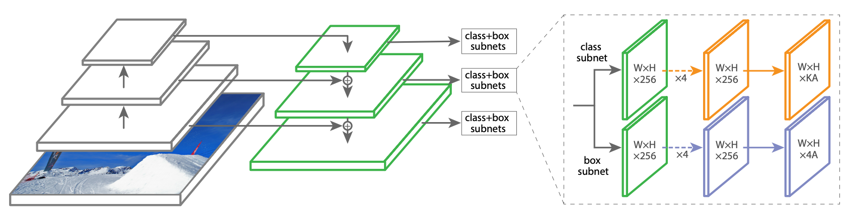
performance stems from two key architectural innovations:
1. Feature Pyramid Network (FPN): FPN equips RetinaNet with the ability to
seamlessly detect objects of all scales, from distant, tiny instances to large,
prominent ones.
2. Focal Loss: This ingenious loss function tackles the common challenge of
imbalanced data by focusing the model's learning on the most crucial and
challenging object examples, leading to enhanced accuracy without compromising
speed.
References
Setup and Imports
Let's install the dependencies and import the necessary modules.
To run this tutorial, you will need to install the following packages:
keras-hubkerasopencv-python
!pip install -q --upgrade keras-hub
!pip install -q --upgrade keras
!pip install -q opencv-python
import os

os.environ["KERAS_BACKEND"] = "jax"  # or "tensorflow" or "torch"
import keras
import keras_hub
import tensorflow as tf
keras-nlp 0.19.0 requires keras-hub==0.19.0, but you have keras-hub 0.26.0 which is incompatible.

WARNING: All log messages before absl::InitializeLog() is called are written to STDERR
E0000 00:00:1775002035.181029    2381 cuda_dnn.cc:8310] Unable to register cuDNN factory: Attempting to register factory for plugin cuDNN when one has already been registered
E0000 00:00:1775002035.187532    2381 cuda_blas.cc:1418] Unable to register cuBLAS factory: Attempting to register factory for plugin cuBLAS when one has already been registered
Helper functions
We download the Pascal VOC 2012 and 2007 datasets using these helper functions, prepare them for the object detection task, and split them into training and validation datasets.
# @title Helper functions
import logging
import multiprocessing
import xml

import tensorflow_datasets as tfds

VOC_2007_URL = (
    "http://host.robots.ox.ac.uk/pascal/VOC/voc2007/VOCtrainval_06-Nov-2007.tar"
)
VOC_2012_URL = (
    "http://host.robots.ox.ac.uk/pascal/VOC/voc2012/VOCtrainval_11-May-2012.tar"
)
VOC_2007_test_URL = (
    "http://host.robots.ox.ac.uk/pascal/VOC/voc2007/VOCtest_06-Nov-2007.tar"
)

# Note that this list doesn't contain the background class. In the
# classification use case, the label is 0 based (aeroplane -> 0), whereas in
# segmentation use case, the 0 is reserved for background, so aeroplane maps to
# 1.
CLASSES = [
    "aeroplane",
    "bicycle",
    "bird",
    "boat",
    "bottle",
    "bus",
    "car",
    "cat",
    "chair",
    "cow",
    "diningtable",
    "dog",
    "horse",
    "motorbike",
    "person",
    "pottedplant",
    "sheep",
    "sofa",
    "train",
    "tvmonitor",
]
COCO_90_CLASS_MAPPING = {
    1: "person",
    2: "bicycle",
    3: "car",
    4: "motorcycle",
    5: "airplane",
    6: "bus",
    7: "train",
    8: "truck",
    9: "boat",
    10: "traffic light",
    11: "fire hydrant",
    13: "stop sign",
    14: "parking meter",
    15: "bench",
    16: "bird",
    17: "cat",
    18: "dog",
    19: "horse",
    20: "sheep",
    21: "cow",
    22: "elephant",
    23: "bear",
    24: "zebra",
    25: "giraffe",
    27: "backpack",
    28: "umbrella",
    31: "handbag",
    32: "tie",
    33: "suitcase",
    34: "frisbee",
    35: "skis",
    36: "snowboard",
    37: "sports ball",
    38: "kite",
    39: "baseball bat",
    40: "baseball glove",
    41: "skateboard",
    42: "surfboard",
    43: "tennis racket",
    44: "bottle",
    46: "wine glass",
    47: "cup",
    48: "fork",
    49: "knife",
    50: "spoon",
    51: "bowl",
    52: "banana",
    53: "apple",
    54: "sandwich",
    55: "orange",
    56: "broccoli",
    57: "carrot",
    58: "hot dog",
    59: "pizza",
    60: "donut",
    61: "cake",
    62: "chair",
    63: "couch",
    64: "potted plant",
    65: "bed",
    67: "dining table",
    70: "toilet",
    72: "tv",
    73: "laptop",
    74: "mouse",
    75: "remote",
    76: "keyboard",
    77: "cell phone",
    78: "microwave",
    79: "oven",
    80: "toaster",
    81: "sink",
    82: "refrigerator",
    84: "book",
    85: "clock",
    86: "vase",
    87: "scissors",
    88: "teddy bear",
    89: "hair drier",
    90: "toothbrush",
}
# This is used to map between string class to index.
CLASS_TO_INDEX = {name: index for index, name in enumerate(CLASSES)}
INDEX_TO_CLASS = {index: name for index, name in enumerate(CLASSES)}


def get_image_ids(data_dir, split):
    """To get image ids from the "train", "eval" or "trainval" files of VOC data."""
    data_file_mapping = {
        "train": "train.txt",
        "eval": "val.txt",
        "trainval": "trainval.txt",
        "test": "test.txt",
    }
    with open(
        os.path.join(data_dir, "ImageSets", "Main", data_file_mapping[split]),
        "r",
    ) as f:
        image_ids = f.read().splitlines()
        logging.info(f"Received {len(image_ids)} images for {split} dataset.")
        return image_ids


def load_images(example):
    """Loads VOC images for segmentation task from the provided paths"""
    image_file_path = example.pop("image/file_path")
    image = tf.io.read_file(image_file_path)
    image = tf.image.decode_jpeg(image)

    example.update(
        {
            "image": image,
        }
    )
    return example


def parse_annotation_data(annotation_file_path):
    """Parse the annotation XML file for the image.

    The annotation contains the metadata, as well as the object bounding box
    information.

    """
    with open(annotation_file_path, "r") as f:
        root = xml.etree.ElementTree.parse(f).getroot()

        size = root.find("size")
        width = int(size.find("width").text)
        height = int(size.find("height").text)
        filename = root.find("filename").text

        objects = []
        for obj in root.findall("object"):
            # Get object's label name.
            label = CLASS_TO_INDEX[obj.find("name").text.lower()]
            bndbox = obj.find("bndbox")
            xmax = int(float(bndbox.find("xmax").text))
            xmin = int(float(bndbox.find("xmin").text))
            ymax = int(float(bndbox.find("ymax").text))
            ymin = int(float(bndbox.find("ymin").text))
            objects.append(
                {
                    "label": label,
                    "bbox": [ymin, xmin, ymax, xmax],
                }
            )

        return {
            "image/filename": filename,
            "width": width,
            "height": height,
            "objects": objects,
        }


def parse_single_image(annotation_file_path):
    """Creates metadata of VOC images and path."""
    data_dir, annotation_file_name = os.path.split(annotation_file_path)
    data_dir = os.path.normpath(os.path.join(data_dir, os.path.pardir))
    image_annotations = parse_annotation_data(annotation_file_path)

    result = {
        "image/file_path": os.path.join(
            data_dir, "JPEGImages", image_annotations["image/filename"]
        )
    }
    result.update(image_annotations)
    # Labels field should be same as the 'object.label'
    labels = list({o["label"] for o in result["objects"]})
    result["labels"] = sorted(labels)
    return result


def build_metadata(data_dir, image_ids):
    """Transpose the metadata which converts from a list of dicts to a dict of lists."""
    # Parallel process all the images.
    annotation_file_paths = [
        os.path.join(data_dir, "Annotations", f"{image_id}.xml")
        for image_id in image_ids
    ]
    pool_size = min(10, len(image_ids))
    with multiprocessing.Pool(pool_size) as p:
        metadata = p.map(parse_single_image, annotation_file_paths)

    keys = [
        "image/filename",
        "image/file_path",
        "labels",
        "width",
        "height",
    ]
    result = {}
    for key in keys:
        values = [value[key] for value in metadata]
        result[key] = values

    # The ragged objects need some special handling
    for key in ["label", "bbox"]:
        values = []
        objects = [value["objects"] for value in metadata]
        for obj_list in objects:
            values.append([o[key] for o in obj_list])
        result["objects/" + key] = values
    return result


def build_dataset_from_metadata(metadata):
    """Builds TensorFlow dataset from the image metadata of VOC dataset."""
    # The objects need some manual conversion to ragged tensor.
    metadata["labels"] = tf.ragged.constant(metadata["labels"])
    metadata["objects/label"] = tf.ragged.constant(metadata["objects/label"])
    metadata["objects/bbox"] = tf.ragged.constant(
        metadata["objects/bbox"], ragged_rank=1
    )

    dataset = tf.data.Dataset.from_tensor_slices(metadata)
    dataset = dataset.map(load_images, num_parallel_calls=tf.data.AUTOTUNE)
    return dataset


def load_voc(
    year="2007",
    split="trainval",
    data_dir="./",
    voc_url=VOC_2007_URL,
):
    extracted_dir = os.path.join("VOCdevkit", f"VOC{year}")
    get_data = keras.utils.get_file(
        fname=os.path.basename(voc_url),
        origin=voc_url,
        cache_dir=data_dir,
        extract=True,
    )
    data_dir = os.path.join(get_data, extracted_dir)
    image_ids = get_image_ids(data_dir, split)
    metadata = build_metadata(data_dir, image_ids)
    dataset = build_dataset_from_metadata(metadata)

    return dataset
Load the dataset
Let's load the training data. Here, we load both the VOC 2007 and 2012 datasets and split them into training and validation sets.
train_ds_2007 = load_voc(
    year="2007",
    split="trainval",
    data_dir="./",
    voc_url=VOC_2007_URL,
)
train_ds_2012 = load_voc(
    year="2012",
    split="trainval",
    data_dir="./",
    voc_url=VOC_2012_URL,
)
eval_ds = load_voc(
    year="2007",
    split="test",
    data_dir="./",
    voc_url=VOC_2007_test_URL,
)
Downloading data from http://host.robots.ox.ac.uk/pascal/VOC/voc2007/VOCtrainval_06-Nov-2007.tar

460032000/460032000 ━━━━━━━━━━━━━━━━━━━━ 16s 0us/step

I0000 00:00:1775002057.754358    2381 gpu_device.cc:2022] Created device /job:localhost/replica:0/task:0/device:GPU:0 with 38482 MB memory:  -> device: 0, name: NVIDIA A100-SXM4-40GB, pci bus id: 0000:00:04.0, compute capability: 8.0

Downloading data from http://host.robots.ox.ac.uk/pascal/VOC/voc2012/VOCtrainval_11-May-2012.tar

1999639040/1999639040 ━━━━━━━━━━━━━━━━━━━━ 65s 0us/step

Downloading data from http://host.robots.ox.ac.uk/pascal/VOC/voc2007/VOCtest_06-Nov-2007.tar

451020800/451020800 ━━━━━━━━━━━━━━━━━━━━ 15s 0us/step
Inference using a pre-trained object detector
Let's begin with the simplest KerasHub API: a pre-trained object detector. In
this example, we will construct an object detector that was pre-trained on the
COCO dataset. We'll use this model to detect objects in a sample image.
The highest-level module in KerasHub is a task. A task is a keras.Model
consisting of a (generally pre-trained) backbone model and task-specific layers.
Here's an example using keras_hub.models.ImageObjectDetector with the
RetinaNet model architecture and ResNet50 as the backbone.
ResNet is a great starting model when constructing an image classification
pipeline. This architecture manages to achieve high accuracy while using a
relatively small number of parameters. If a ResNet isn't powerful enough for the
task you are hoping to solve, be sure to check out KerasHub's other available
backbones here https://keras.io/keras_hub/presets/
object_detector = keras_hub.models.ImageObjectDetector.from_preset(
    "retinanet_resnet50_fpn_coco"
)
object_detector.summary()
Downloading from https://www.kaggle.com/api/v1/models/keras/retinanet/keras/retinanet_resnet50_fpn_coco/4/download/config.json...
0%| | 0.00/1.59k [00:00<?, ?B/s]
100%|█████████████████████████████████████████████████████████████████████████████████████████████████████████████████████████████████████████████████████████████████████████████████| 1.59k/1.59k [00:00<00:00, 3.14MB/s]
Downloading from https://www.kaggle.com/api/v1/models/keras/retinanet/keras/retinanet_resnet50_fpn_coco/4/download/task.json...
0%| | 0.00/8.54k [00:00<?, ?B/s]
100%|█████████████████████████████████████████████████████████████████████████████████████████████████████████████████████████████████████████████████████████████████████████████████| 8.54k/8.54k [00:00<00:00, 18.1MB/s]
Downloading from https://www.kaggle.com/api/v1/models/keras/retinanet/keras/retinanet_resnet50_fpn_coco/4/download/task.weights.h5...
0%| | 0.00/131M [00:00<?, ?B/s]
1%|█▎ | 1.00M/131M [00:00<00:22, 6.09MB/s]
5%|████████▏ | 6.00M/131M [00:00<00:05, 25.2MB/s]
13%|███████████████████████▏ | 17.0M/131M [00:00<00:02, 47.2MB/s]
21%|██████████████████████████████████████▏ | 28.0M/131M [00:00<00:01, 65.4MB/s]
27%|███████████████████████████████████████████████▋ | 35.0M/131M [00:00<00:01, 57.2MB/s]
34%|█████████████████████████████████████████████████████████████▎ | 45.0M/131M [00:00<00:01, 67.8MB/s]
42%|██████████████████████████████████████████████████████████████████████████▉ | 55.0M/131M [00:00<00:01, 77.1MB/s]
51%|███████████████████████████████████████████████████████████████████████████████████████████▏ | 67.0M/131M [00:01<00:00, 73.6MB/s]
60%|███████████████████████████████████████████████████████████████████████████████████████████████████████████▌ | 79.0M/131M [00:01<00:00, 84.8MB/s]
69%|██████████████████████████████████████████████████████████████████████████████████████████████████████████████████████████▌ | 90.0M/131M [00:01<00:00, 89.0MB/s]
80%|███████████████████████████████████████████████████████████████████████████████████████████████████████████████████████████████████████████████▏ | 104M/131M [00:01<00:00, 104MB/s]
89%|██████████████████████████████████████████████████████████████████████████████████████████████████████████████████████████████████████████████████████████████▊ | 116M/131M [00:01<00:00, 99.7MB/s]
96%|████████████████████████████████████████████████████████████████████████████████████████████████████████████████████████████████████████████████████████████████████████████▌ | 126M/131M [00:01<00:00, 86.8MB/s]
100%|███████████████████████████████████████████████████████████████████████████████████████████████████████████████████████████████████████████████████████████████████████████████████| 131M/131M [00:01<00:00, 74.9MB/s]
Downloading from https://www.kaggle.com/api/v1/models/keras/retinanet/keras/retinanet_resnet50_fpn_coco/4/download/model.weights.h5...
0%| | 0.00/105M [00:00<?, ?B/s]
1%|█▋ | 1.00M/105M [00:00<00:19, 5.66MB/s]
4%|██████▊ | 4.00M/105M [00:00<00:06, 16.8MB/s]
13%|███████████████████████▋ | 14.0M/105M [00:00<00:01, 50.3MB/s]
20%|███████████████████████████████████▌ | 21.0M/105M [00:00<00:01, 56.7MB/s]
32%|█████████████████████████████████████████████████████████▌ | 34.0M/105M [00:00<00:01, 67.5MB/s]
44%|█████████████████████████████████████████████████████████████████████████████▉ | 46.0M/105M [00:00<00:00, 82.9MB/s]
52%|█████████████████████████████████████████████████████████████████████████████████████████████▏ | 55.0M/105M [00:00<00:00, 82.6MB/s]
61%|████████████████████████████████████████████████████████████████████████████████████████████████████████████▍ | 64.0M/105M [00:01<00:00, 73.7MB/s]
72%|████████████████████████████████████████████████████████████████████████████████████████████████████████████████████████████████▋ | 76.0M/105M [00:01<00:00, 84.3MB/s]
83%|███████████████████████████████████████████████████████████████████████████████████████████████████████████████████████████████████████████████████▎ | 87.0M/105M [00:01<00:00, 81.8MB/s]
95%|██████████████████████████████████████████████████████████████████████████████████████████████████████████████████████████████████████████████████████████████████████████▎ | 100M/105M [00:01<00:00, 92.1MB/s]
100%|███████████████████████████████████████████████████████████████████████████████████████████████████████████████████████████████████████████████████████████████████████████████████| 105M/105M [00:01<00:00, 75.6MB/s]
Preprocessor: "retina_net_object_detector_preprocessor"
┏━━━━━━━━━━━━━━━━━━━━━━━━━━━━━━━━━━━━━━━━━━━━━━━━━━━━━━━━━━━━━━━┳━━━━━━━━━━━━━━━━━━━━━━━━━━━━━━━━━━━━━━━━━━┓
┃ Layer (type)                                                  ┃                                   Config ┃
┡━━━━━━━━━━━━━━━━━━━━━━━━━━━━━━━━━━━━━━━━━━━━━━━━━━━━━━━━━━━━━━━╇━━━━━━━━━━━━━━━━━━━━━━━━━━━━━━━━━━━━━━━━━━┩
│ retina_net_image_converter (RetinaNetImageConverter)          │                   Image size: (800, 800) │
└───────────────────────────────────────────────────────────────┴──────────────────────────────────────────┘
Model: "retina_net_object_detector"
┏━━━━━━━━━━━━━━━━━━━━━━━━━━━━━━━┳━━━━━━━━━━━━━━━━━━━━━━━━━━━┳━━━━━━━━━━━━━━━━━┳━━━━━━━━━━━━━━━━━━━━━━━━━━━━┓
┃ Layer (type)                  ┃ Output Shape              ┃         Param # ┃ Connected to               ┃
┡━━━━━━━━━━━━━━━━━━━━━━━━━━━━━━━╇━━━━━━━━━━━━━━━━━━━━━━━━━━━╇━━━━━━━━━━━━━━━━━╇━━━━━━━━━━━━━━━━━━━━━━━━━━━━┩
│ images (InputLayer)           │ (None, None, None, 3)     │               0 │ -                          │
├───────────────────────────────┼───────────────────────────┼─────────────────┼────────────────────────────┤
│ retina_net_backbone           │ [(None, None, None, 256), │      27,429,824 │ images[0][0]               │
│ (RetinaNetBackbone)           │ (None, None, None, 256),  │                 │                            │
│                               │ (None, None, None, 256),  │                 │                            │
│                               │ (None, None, None, 256),  │                 │                            │
│                               │ (None, None, None, 256)]  │                 │                            │
├───────────────────────────────┼───────────────────────────┼─────────────────┼────────────────────────────┤
│ box_head (PredictionHead)     │ (None, None, None, 36)    │       2,443,300 │ retina_net_backbone[0][0], │
│                               │                           │                 │ retina_net_backbone[0][1], │
│                               │                           │                 │ retina_net_backbone[0][2], │
│                               │                           │                 │ retina_net_backbone[0][3], │
│                               │                           │                 │ retina_net_backbone[0][4]  │
├───────────────────────────────┼───────────────────────────┼─────────────────┼────────────────────────────┤
│ classification_head           │ (None, None, None, 819)   │       4,248,115 │ retina_net_backbone[0][0], │
│ (PredictionHead)              │                           │                 │ retina_net_backbone[0][1], │
│                               │                           │                 │ retina_net_backbone[0][2], │
│                               │                           │                 │ retina_net_backbone[0][3], │
│                               │                           │                 │ retina_net_backbone[0][4]  │
├───────────────────────────────┼───────────────────────────┼─────────────────┼────────────────────────────┤
│ box_pred_P3 (Reshape)         │ (None, None, 4)           │               0 │ box_head[0][0]             │
├───────────────────────────────┼───────────────────────────┼─────────────────┼────────────────────────────┤
│ box_pred_P4 (Reshape)         │ (None, None, 4)           │               0 │ box_head[1][0]             │
├───────────────────────────────┼───────────────────────────┼─────────────────┼────────────────────────────┤
│ box_pred_P5 (Reshape)         │ (None, None, 4)           │               0 │ box_head[2][0]             │
├───────────────────────────────┼───────────────────────────┼─────────────────┼────────────────────────────┤
│ box_pred_P6 (Reshape)         │ (None, None, 4)           │               0 │ box_head[3][0]             │
├───────────────────────────────┼───────────────────────────┼─────────────────┼────────────────────────────┤
│ box_pred_P7 (Reshape)         │ (None, None, 4)           │               0 │ box_head[4][0]             │
├───────────────────────────────┼───────────────────────────┼─────────────────┼────────────────────────────┤
│ cls_pred_P3 (Reshape)         │ (None, None, 91)          │               0 │ classification_head[0][0]  │
├───────────────────────────────┼───────────────────────────┼─────────────────┼────────────────────────────┤
│ cls_pred_P4 (Reshape)         │ (None, None, 91)          │               0 │ classification_head[1][0]  │
├───────────────────────────────┼───────────────────────────┼─────────────────┼────────────────────────────┤
│ cls_pred_P5 (Reshape)         │ (None, None, 91)          │               0 │ classification_head[2][0]  │
├───────────────────────────────┼───────────────────────────┼─────────────────┼────────────────────────────┤
│ cls_pred_P6 (Reshape)         │ (None, None, 91)          │               0 │ classification_head[3][0]  │
├───────────────────────────────┼───────────────────────────┼─────────────────┼────────────────────────────┤
│ cls_pred_P7 (Reshape)         │ (None, None, 91)          │               0 │ classification_head[4][0]  │
├───────────────────────────────┼───────────────────────────┼─────────────────┼────────────────────────────┤
│ bbox_regression (Concatenate) │ (None, None, 4)           │               0 │ box_pred_P3[0][0],         │
│                               │                           │                 │ box_pred_P4[0][0],         │
│                               │                           │                 │ box_pred_P5[0][0],         │
│                               │                           │                 │ box_pred_P6[0][0],         │
│                               │                           │                 │ box_pred_P7[0][0]          │
├───────────────────────────────┼───────────────────────────┼─────────────────┼────────────────────────────┤
│ cls_logits (Concatenate)      │ (None, None, 91)          │               0 │ cls_pred_P3[0][0],         │
│                               │                           │                 │ cls_pred_P4[0][0],         │
│                               │                           │                 │ cls_pred_P5[0][0],         │
│                               │                           │                 │ cls_pred_P6[0][0],         │
│                               │                           │                 │ cls_pred_P7[0][0]          │
└───────────────────────────────┴───────────────────────────┴─────────────────┴────────────────────────────┘
Total params: 34,121,239 (130.16 MB)
Trainable params: 34,068,119 (129.96 MB)
Non-trainable params: 53,120 (207.50 KB)
Preprocessing Layers
Let's define the below preprocessing layers:
- Resizing Layer: Resizes the image and maintains the aspect ratio by applying
padding when
pad_to_aspect_ratio=True. Also, sets the default bounding box format for representing the data. - Max Bounding Box Layer: Limits the maximum number of bounding boxes per image.
image_size = (800, 800)
batch_size = 4
bbox_format = "yxyx"
epochs = 5

resizing = keras.layers.Resizing(
    height=image_size[0],
    width=image_size[1],
    interpolation="bilinear",
    pad_to_aspect_ratio=True,
    bounding_box_format=bbox_format,
)

max_box_layer = keras.layers.MaxNumBoundingBoxes(
    max_number=100, bounding_box_format=bbox_format
)
Predict and Visualize
Next, let's obtain predictions from our object detector by loading the image and visualizing them. We'll apply the preprocessing pipeline defined in the preprocessing layers step.
filepath = keras.utils.get_file(
    origin="http://images.cocodataset.org/val2017/000000039769.jpg",
)
image = keras.utils.load_img(filepath)
image = keras.ops.cast(image, "float32")
image = keras.ops.expand_dims(image, axis=0)

predictions = object_detector.predict(image, batch_size=1)

keras.visualization.plot_bounding_box_gallery(
    resizing(image),  # resize image as per prediction preprocessing pipeline
    bounding_box_format=bbox_format,
    y_pred=predictions,
    scale=4,
    class_mapping=COCO_90_CLASS_MAPPING,
)
Downloading data from http://images.cocodataset.org/val2017/000000039769.jpg

1/1 ━━━━━━━━━━━━━━━━━━━━ 8s 8s/step

Fine tuning a pretrained object detector
In this guide, we'll assemble a full training pipeline for a KerasHub RetinaNet
object detection model. This includes data loading, augmentation, training, and
inference using Pascal VOC 2007 & 2012 dataset!
TFDS Preprocessing
This preprocessing step prepares the TFDS dataset for object detection. It includes: - Merging the Pascal VOC 2007 and 2012 datasets. - Resizing all images to a resolution of 800x800 pixels. - Limiting the number of bounding boxes per image to a maximum of 100. - Finally, the resulting dataset is batched into sets of 4 images and bounding box annotations.
def decode_custom_tfds(record):
    """Decodes a custom TFDS record into a dictionary.

    Args:
      record: A dictionary representing a single TFDS record.

    Returns:
      A dictionary with "images" and "bounding_boxes".
    """
    image = record["image"]
    boxes = record["objects/bbox"]
    labels = record["objects/label"]

    bounding_boxes = {"boxes": boxes, "labels": labels}

    return {"images": image, "bounding_boxes": bounding_boxes}


def convert_to_tuple(record):
    """Converts a decoded TFDS record to a tuple for KerasHub.

    Args:
      record: A dictionary returned by `decode_custom_tfds`.

    Returns:
      A tuple (image, bounding_boxes).
    """
    return record["images"], {
        "boxes": record["bounding_boxes"]["boxes"],
        "labels": record["bounding_boxes"]["labels"],
    }


def preprocess_tfds(ds, resizing, max_box_layer, batch_size):
    """Preprocesses a TFDS dataset for object detection.

    Args:
        ds: The TFDS dataset.
        resizing: A resizing function.
        max_box_layer: A max box processing function.
        batch_size: The batch size.

    Returns:
      A preprocessed TFDS dataset.
    """
    ds = ds.map(resizing, num_parallel_calls=tf.data.AUTOTUNE)
    ds = ds.map(max_box_layer, num_parallel_calls=tf.data.AUTOTUNE)
    ds = ds.batch(batch_size, drop_remainder=True)
    return ds
Now concatenate both 2007 and 2012 VOC data
train_ds = train_ds_2007.concatenate(train_ds_2012)
train_ds = train_ds.map(decode_custom_tfds, num_parallel_calls=tf.data.AUTOTUNE)
train_ds = preprocess_tfds(train_ds, resizing, max_box_layer, batch_size)
Load the eval data
eval_ds = eval_ds.map(decode_custom_tfds, num_parallel_calls=tf.data.AUTOTUNE)
eval_ds = preprocess_tfds(eval_ds, resizing, max_box_layer, batch_size)
Let's visualize a batch of training data
record = next(iter(train_ds.shuffle(100).take(1)))
keras.visualization.plot_bounding_box_gallery(
    record["images"],
    bounding_box_format=bbox_format,
    y_true=record["bounding_boxes"],
    scale=3,
    rows=2,
    cols=2,
    class_mapping=INDEX_TO_CLASS,
)

Decode TFDS records to a tuple for KerasHub
train_ds = train_ds.map(convert_to_tuple, num_parallel_calls=tf.data.AUTOTUNE)
train_ds = train_ds.prefetch(tf.data.AUTOTUNE)

eval_ds = eval_ds.map(convert_to_tuple, num_parallel_calls=tf.data.AUTOTUNE)
eval_ds = eval_ds.prefetch(tf.data.AUTOTUNE)
Configure RetinaNet Model
Configure the model with backbone, num_classes and preprocessor.
Use callbacks for recording logs and saving checkpoints.
def get_callbacks(experiment_path):
    """Creates a list of callbacks for model training.

    Args:
      experiment_path (str): Path to the experiment directory.

    Returns:
      List of keras callback instances.
    """
    tb_logs_path = os.path.join(experiment_path, "logs")
    backup_path = os.path.join(experiment_path, "backup")
    ckpt_path = os.path.join(experiment_path, "weights")
    return [
        keras.callbacks.BackupAndRestore(backup_path, delete_checkpoint=False),
        keras.callbacks.TensorBoard(
            tb_logs_path,
            update_freq=1,
        ),
        keras.callbacks.ModelCheckpoint(
            os.path.join(ckpt_path, "{epoch:04d}-{val_loss:.2f}.weights.h5"),
            save_best_only=True,
            save_weights_only=True,
            verbose=1,
        ),
    ]
Load backbone weights and preprocessor config
Let's use the "retinanet_resnet50_fpn_coco" pretrained weights as the backbone
model, applying its predefined configuration from the preprocessor of the
"retinanet_resnet50_fpn_coco" preset.
Define a RetinaNet object detector model with the backbone and preprocessor
specified above, and set num_classes to 20 to represent the object categories
from Pascal VOC.
Finally, compile the model using Mean Absolute Error (MAE) as the box loss.
backbone = keras_hub.models.Backbone.from_preset("retinanet_resnet50_fpn_coco")

preprocessor = keras_hub.models.RetinaNetObjectDetectorPreprocessor.from_preset(
    "retinanet_resnet50_fpn_coco"
)
model = keras_hub.models.RetinaNetObjectDetector(
    backbone=backbone, num_classes=len(CLASSES), preprocessor=preprocessor
)
model.compile(box_loss=keras.losses.MeanAbsoluteError(reduction="sum"))
Downloading from https://www.kaggle.com/api/v1/models/keras/retinanet/keras/retinanet_resnet50_fpn_coco/4/download/preprocessor.json...
0%| | 0.00/1.84k [00:00<?, ?B/s]
100%|█████████████████████████████████████████████████████████████████████████████████████████████████████████████████████████████████████████████████████████████████████████████████| 1.84k/1.84k [00:00<00:00, 4.87MB/s]
Train the model
Now that the object detector model is compiled, let's train it using the training and validation data we created earlier. For demonstration purposes, we have used a small number of epochs. You can increase the number of epochs to achieve better results.
Note: The model is trained on an L4 GPU. Training for 5 epochs on a T4 GPU takes approximately 7 hours.
model.fit(
    train_ds,
    epochs=epochs,
    validation_data=eval_ds,
    callbacks=get_callbacks("fine_tuning"),
)
Epoch 1/5

4137/4137 ━━━━━━━━━━━━━━━━━━━━ 0s 110ms/step - bbox_regression_loss: 1.1873 - cls_logits_loss: 95.7444 - loss: 96.9318

Epoch 1: val_loss improved from None to 0.31972, saving model to fine_tuning/weights/0001-0.32.weights.h5

Epoch 1: finished saving model to fine_tuning/weights/0001-0.32.weights.h5

4137/4137 ━━━━━━━━━━━━━━━━━━━━ 534s 119ms/step - bbox_regression_loss: 0.4609 - cls_logits_loss: 13.6850 - loss: 14.1459 - val_bbox_regression_loss: 0.1833 - val_cls_logits_loss: 0.1364 - val_loss: 0.3197

Epoch 2/5

4137/4137 ━━━━━━━━━━━━━━━━━━━━ 0s 110ms/step - bbox_regression_loss: 0.1946 - cls_logits_loss: 0.1243 - loss: 0.3189

Epoch 2: val_loss improved from 0.31972 to 0.25071, saving model to fine_tuning/weights/0002-0.25.weights.h5

Epoch 2: finished saving model to fine_tuning/weights/0002-0.25.weights.h5

4137/4137 ━━━━━━━━━━━━━━━━━━━━ 491s 119ms/step - bbox_regression_loss: 0.1863 - cls_logits_loss: 0.1163 - loss: 0.3026 - val_bbox_regression_loss: 0.1518 - val_cls_logits_loss: 0.0989 - val_loss: 0.2507

Epoch 3/5

4137/4137 ━━━━━━━━━━━━━━━━━━━━ 0s 111ms/step - bbox_regression_loss: 0.1741 - cls_logits_loss: 0.0943 - loss: 0.2684

Epoch 3: val_loss improved from 0.25071 to 0.20826, saving model to fine_tuning/weights/0003-0.21.weights.h5

Epoch 3: finished saving model to fine_tuning/weights/0003-0.21.weights.h5

4137/4137 ━━━━━━━━━━━━━━━━━━━━ 495s 120ms/step - bbox_regression_loss: 0.1695 - cls_logits_loss: 0.0902 - loss: 0.2597 - val_bbox_regression_loss: 0.1298 - val_cls_logits_loss: 0.0784 - val_loss: 0.2083

Epoch 4/5

4137/4137 ━━━━━━━━━━━━━━━━━━━━ 0s 110ms/step - bbox_regression_loss: 0.1553 - cls_logits_loss: 0.0727 - loss: 0.2280

Epoch 4: val_loss improved from 0.20826 to 0.20306, saving model to fine_tuning/weights/0004-0.20.weights.h5

Epoch 4: finished saving model to fine_tuning/weights/0004-0.20.weights.h5

4137/4137 ━━━━━━━━━━━━━━━━━━━━ 490s 118ms/step - bbox_regression_loss: 0.1486 - cls_logits_loss: 0.0701 - loss: 0.2187 - val_bbox_regression_loss: 0.1437 - val_cls_logits_loss: 0.0593 - val_loss: 0.2031

Epoch 5/5

4137/4137 ━━━━━━━━━━━━━━━━━━━━ 0s 111ms/step - bbox_regression_loss: 0.1297 - cls_logits_loss: 0.0566 - loss: 0.1863

Epoch 5: val_loss improved from 0.20306 to 0.17988, saving model to fine_tuning/weights/0005-0.18.weights.h5

Epoch 5: finished saving model to fine_tuning/weights/0005-0.18.weights.h5

4137/4137 ━━━━━━━━━━━━━━━━━━━━ 492s 119ms/step - bbox_regression_loss: 0.1269 - cls_logits_loss: 0.0547 - loss: 0.1817 - val_bbox_regression_loss: 0.1297 - val_cls_logits_loss: 0.0501 - val_loss: 0.1799

<keras.src.callbacks.history.History at 0x7f1cbb73a910>
Prediction on evaluation data
Let's make predictions using our model on the evaluation dataset.
images, y_true = next(iter(eval_ds.shuffle(50).take(1)))
y_pred = model.predict(images)
1/1 ━━━━━━━━━━━━━━━━━━━━ 7s 7s/step
Plot the predictions
keras.visualization.plot_bounding_box_gallery(
    images,
    bounding_box_format=bbox_format,
    y_true=y_true,
    y_pred=y_pred,
    scale=3,
    rows=2,
    cols=2,
    class_mapping=INDEX_TO_CLASS,
)

Custom training object detector
Additionally, you can customize the object detector by modifying the image converter, selecting a different image encoder, etc.
Image Converter
The RetinaNetImageConverter class prepares images for use with the RetinaNet
object detection model. Here's what it does:
- Scaling and Offsetting
- ImageNet Normalization
- Resizing
image_converter = keras_hub.layers.RetinaNetImageConverter(scale=1 / 255)

preprocessor = keras_hub.models.RetinaNetObjectDetectorPreprocessor(
    image_converter=image_converter
)
Image Encoder and RetinaNet Backbone
The image encoder, while typically initialized with pre-trained weights (e.g., from ImageNet), can also be instantiated without them. This results in the image encoder (and, consequently, the entire object detection network built upon it) having randomly initialized weights.
Here we load pre-trained ResNet50 model. This will serve as the base for extracting image features.
And then build the RetinaNet Feature Pyramid Network (FPN) on top of the ResNet50 backbone. The FPN creates multi-scale feature maps for better object detection at different sizes.
Note:
use_p5: If True, the output of the last backbone layer (typically P5 in an
FPN) is used as input to create higher-level feature maps (e.g., P6, P7)
through additional convolutional layers. If False, the original P5 feature
map from the backbone is directly used as input for creating the coarser levels,
bypassing any further processing of P5 within the feature pyramid. Defaults to
False.
image_encoder = keras_hub.models.Backbone.from_preset("resnet_50_imagenet")

backbone = keras_hub.models.RetinaNetBackbone(
    image_encoder=image_encoder, min_level=3, max_level=5, use_p5=True
)
Train and visualize RetinaNet model
Note: Training the model (for demonstration purposes only 5 epochs). In a real scenario, you would train for many more epochs (often hundreds) to achieve good results.
model = keras_hub.models.RetinaNetObjectDetector(
    backbone=backbone,
    num_classes=len(CLASSES),
    preprocessor=preprocessor,
    use_prediction_head_norm=True,
)
model.compile(
    optimizer=keras.optimizers.Adam(learning_rate=0.001),
    box_loss=keras.losses.MeanAbsoluteError(reduction="sum"),
)

model.fit(
    train_ds,
    epochs=epochs,
    validation_data=eval_ds,
    callbacks=get_callbacks("custom_training"),
)

images, y_true = next(iter(eval_ds.shuffle(50).take(1)))
y_pred = model.predict(images)

keras.visualization.plot_bounding_box_gallery(
    images,
    bounding_box_format=bbox_format,
    y_true=y_true,
    y_pred=y_pred,
    scale=3,
    rows=2,
    cols=2,
    class_mapping=INDEX_TO_CLASS,
)
Epoch 1/5

4137/4137 ━━━━━━━━━━━━━━━━━━━━ 0s 109ms/step - bbox_regression_loss: 0.2777 - cls_logits_loss: 5.8220 - loss: 6.0997

Epoch 1: val_loss improved from None to 0.28498, saving model to custom_training/weights/0001-0.28.weights.h5

Epoch 1: finished saving model to custom_training/weights/0001-0.28.weights.h5

4137/4137 ━━━━━━━━━━━━━━━━━━━━ 521s 118ms/step - bbox_regression_loss: 0.2125 - cls_logits_loss: 0.8302 - loss: 1.0427 - val_bbox_regression_loss: 0.1502 - val_cls_logits_loss: 0.1348 - val_loss: 0.2850

Epoch 2/5

4137/4137 ━━━━━━━━━━━━━━━━━━━━ 0s 109ms/step - bbox_regression_loss: 0.1528 - cls_logits_loss: 0.1169 - loss: 0.2697

Epoch 2: val_loss improved from 0.28498 to 0.25430, saving model to custom_training/weights/0002-0.25.weights.h5

Epoch 2: finished saving model to custom_training/weights/0002-0.25.weights.h5

4137/4137 ━━━━━━━━━━━━━━━━━━━━ 486s 118ms/step - bbox_regression_loss: 0.1453 - cls_logits_loss: 0.1176 - loss: 0.2629 - val_bbox_regression_loss: 0.1315 - val_cls_logits_loss: 0.1228 - val_loss: 0.2543

Epoch 3/5

4137/4137 ━━━━━━━━━━━━━━━━━━━━ 0s 109ms/step - bbox_regression_loss: 0.1255 - cls_logits_loss: 0.0995 - loss: 0.2250

Epoch 3: val_loss improved from 0.25430 to 0.22651, saving model to custom_training/weights/0003-0.23.weights.h5

Epoch 3: finished saving model to custom_training/weights/0003-0.23.weights.h5

4137/4137 ━━━━━━━━━━━━━━━━━━━━ 485s 117ms/step - bbox_regression_loss: 0.1215 - cls_logits_loss: 0.0987 - loss: 0.2202 - val_bbox_regression_loss: 0.1270 - val_cls_logits_loss: 0.0995 - val_loss: 0.2265

Epoch 4/5

4137/4137 ━━━━━━━━━━━━━━━━━━━━ 0s 109ms/step - bbox_regression_loss: 0.1095 - cls_logits_loss: 0.0803 - loss: 0.1898

Epoch 4: val_loss improved from 0.22651 to 0.18972, saving model to custom_training/weights/0004-0.19.weights.h5

Epoch 4: finished saving model to custom_training/weights/0004-0.19.weights.h5

4137/4137 ━━━━━━━━━━━━━━━━━━━━ 485s 117ms/step - bbox_regression_loss: 0.1071 - cls_logits_loss: 0.0801 - loss: 0.1872 - val_bbox_regression_loss: 0.1058 - val_cls_logits_loss: 0.0839 - val_loss: 0.1897

Epoch 5/5

4137/4137 ━━━━━━━━━━━━━━━━━━━━ 0s 109ms/step - bbox_regression_loss: 0.0978 - cls_logits_loss: 0.0663 - loss: 0.1641

Epoch 5: val_loss did not improve from 0.18972

1/1 ━━━━━━━━━━━━━━━━━━━━ 7s 7s/step

Conclusion
In this tutorial, you learned how to custom train and fine-tune the RetinaNet object detector.
You can experiment with different existing backbones trained on ImageNet as the image encoder, or you can fine-tune your own backbone.
This configuration is equivalent to training the model from scratch, as opposed to fine-tuning a pre-trained model.
Training from scratch generally requires significantly more data and computational resources to achieve performance comparable to fine-tuning.
To achieve better results when fine-tuning the model, you can increase the number of epochs and experiment with different hyperparameter values. In addition to the training data used here, you can also use other object detection datasets, but keep in mind that custom training these requires high GPU memory.