Node Classification with Graph Neural Networks
Author: Khalid Salama
Date created: 2021/05/30
Last modified: 2021/05/30
Description: Implementing a graph neural network model for predicting the topic of a paper given its citations.

Introduction
Many datasets in various machine learning (ML) applications have structural relationships between their entities, which can be represented as graphs. Such application includes social and communication networks analysis, traffic prediction, and fraud detection. Graph representation Learning aims to build and train models for graph datasets to be used for a variety of ML tasks.
This example demonstrate a simple implementation of a Graph Neural Network (GNN) model. The model is used for a node prediction task on the Cora dataset to predict the subject of a paper given its words and citations network.
Note that, we implement a Graph Convolution Layer from scratch to provide better understanding of how they work. However, there is a number of specialized TensorFlow-based libraries that provide rich GNN APIs, such as Spectral, StellarGraph, and GraphNets.
Setup
import os

# Choose backend: "jax", "torch", or "tensorflow"
os.environ["KERAS_BACKEND"] = "tensorflow"
import pandas as pd
import numpy as np
import networkx as nx
import matplotlib

# matplotlib.use("Agg")  # Use non-interactive backend
import matplotlib.pyplot as plt
import keras
from keras import layers, ops

keras.utils.set_random_seed(42)
rng = np.random.default_rng(42)
Prepare and Download the Dataset
The Cora dataset consists of 2,708 scientific papers classified into one of seven classes.
The citation network consists of 5,429 links. Each paper has a binary word vector of size
1,433, indicating the presence of a corresponding word.
The dataset has two tap-separated files: cora.cites and cora.content.
- The
cora.citesincludes the citation records with two columns:cited_paper_id(target) andciting_paper_id(source). - The
cora.contentincludes the paper content records with 1,435 columns:paper_id,subject, and 1,433 binary features.
zip_file = keras.utils.get_file(
    fname="cora.tgz",
    origin="https://linqs-data.soe.ucsc.edu/public/lbc/cora.tgz",
    extract=True,
)
data_dir = os.path.join(os.path.dirname(zip_file), "cora_extracted", "cora")
Process and visualize the dataset
citations = pd.read_csv(
    os.path.join(data_dir, "cora.cites"),
    sep="\t",
    header=None,
    names=["target", "source"],
)
print("Citations shape:", citations.shape)

citations.sample(frac=1).head()  # display a sample of the `citations` DataFrame
Citations shape: (5429, 2)
| target | source | |
|---|---|---|
| 79 | 35 | 263498 |
| 3161 | 45605 | 503871 |
| 1643 | 9581 | 1130780 |
| 167 | 40 | 1114442 |
| 439 | 1365 | 22835 |
Now let's load the papers data into a Pandas DataFrame.
column_names = ["paper_id"] + [f"term_{idx}" for idx in range(1433)] + ["subject"]
papers = pd.read_csv(
    os.path.join(data_dir, "cora.content"),
    sep="\t",
    header=None,
    names=column_names,
)
print("Papers shape:", papers.shape)
Papers shape: (2708, 1435)
Now we display a sample of the papers DataFrame. The DataFrame includes the paper_id
and the subject columns, as well as 1,433 binary column representing whether a term exists
in the paper or not.
print(papers.sample(5).T)
             1026             405                     1202             461   \
paper_id    93273            16470                   95597           919885
term_0          0                0                       0                0
term_1          0                0                       0                0
term_2          0                0                       0                0
term_3          0                0                       1                0
...           ...              ...                     ...              ...
term_1429       0                0                       0                0
term_1430       0                0                       0                0
term_1431       0                0                       0                0
term_1432       0                0                       0                0
subject    Theory  Neural_Networks  Reinforcement_Learning  Neural_Networks

                            2285
paper_id                  643695
term_0                         0
term_1                         0
term_2                         0
term_3                         0
...                          ...
term_1429                      0
term_1430                      0
term_1431                      0
term_1432                      0
subject    Probabilistic_Methods

[1435 rows x 5 columns]
Let's display the count of the papers in each subject.
print(papers.subject.value_counts())
subject
Neural_Networks           818
Probabilistic_Methods     426
Genetic_Algorithms        418
Theory                    351
Case_Based                298
Reinforcement_Learning    217
Rule_Learning             180
Name: count, dtype: int64
We convert the paper ids and the subjects into zero-based indices.
class_values = sorted(papers["subject"].unique())
class_idx = {name: id for id, name in enumerate(class_values)}
num_classes = len(class_values)
paper_idx = {name: idx for idx, name in enumerate(sorted(papers["paper_id"].unique()))}

papers["paper_id"] = papers["paper_id"].apply(lambda name: paper_idx[name])
citations["source"] = citations["source"].apply(lambda name: paper_idx[name])
citations["target"] = citations["target"].apply(lambda name: paper_idx[name])
papers["subject"] = papers["subject"].apply(lambda value: class_idx[value])
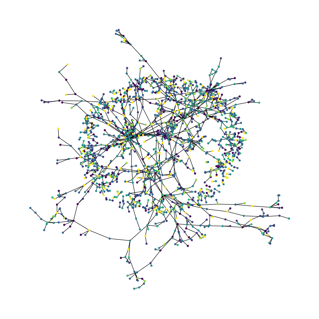
Now let's visualize the citation graph. Each node in the graph represents a paper, and the color of the node corresponds to its subject. Note that we only show a sample of the papers in the dataset.
plt.figure(figsize=(10, 10))
colors = papers["subject"].tolist()
cora_graph = nx.from_pandas_edgelist(citations.sample(n=1500))
subjects = list(papers[papers["paper_id"].isin(list(cora_graph.nodes))]["subject"])
nx.draw_spring(cora_graph, node_size=15, node_color=subjects)
plt.show()
Split the dataset into stratified train, validation, and test sets
train_ids, val_ids, test_ids = [], [], []
for cls, group in papers.groupby("subject"):
    ids = group["paper_id"].to_numpy().copy()
    rng.shuffle(ids)

    n = len(ids)
    n_train = int(0.50 * n)
    n_val = int(0.15 * n)

    train_ids.append(ids[:n_train])
    val_ids.append(ids[n_train : n_train + n_val])
    test_ids.append(ids[n_train + n_val :])

train_indices = np.concatenate(train_ids).astype("int32")
val_indices = np.concatenate(val_ids).astype("int32")
test_indices = np.concatenate(test_ids).astype("int32")

labels_by_id = papers.sort_values("paper_id")["subject"].to_numpy().astype("int32")
train_labels = labels_by_id[train_indices]
val_labels = labels_by_id[val_indices]
test_labels = labels_by_id[test_indices]

# Shuffle training nodes (good practice)
perm = rng.permutation(len(train_indices))
train_indices = train_indices[perm]
train_labels = train_labels[perm]

print("Train idx/labels:", train_indices.shape, train_labels.shape)
print("Val   idx/labels:", val_indices.shape, val_labels.shape)
print("Test  idx/labels:", test_indices.shape, test_labels.shape)
Train idx/labels: (1353,) (1353,)
Val   idx/labels: (402,) (402,)
Test  idx/labels: (953,) (953,)
Implement Train and Evaluate Experiment
hidden_units = [32, 32]
dropout_rate = 0.5
learning_rate = 0.01
num_epochs = 300
batch_size = 256
This function compiles and trains an input model using the given training data.
def run_experiment(model, x_train, y_train, x_val, y_val):
    model.compile(
        optimizer=keras.optimizers.Adam(learning_rate=learning_rate),
        loss=keras.losses.SparseCategoricalCrossentropy(from_logits=True),
        metrics=[keras.metrics.SparseCategoricalAccuracy(name="acc")],
    )
    early_stopping = keras.callbacks.EarlyStopping(
        monitor="val_loss",
        mode="min",
        patience=50,
        restore_best_weights=True,
    )
    history = model.fit(
        x=x_train,
        y=y_train,
        validation_data=(x_val, y_val),
        epochs=num_epochs,
        batch_size=batch_size,
        callbacks=[early_stopping],
        verbose=2,
    )
    return history
This function displays the loss and accuracy curves of the model during training.
def display_learning_curves(history, title=None):
    fig, (ax1, ax2) = plt.subplots(1, 2, figsize=(15, 5))
    if title:
        fig.suptitle(title)

    ax1.plot(history.history["loss"])
    ax1.plot(history.history["val_loss"])
    ax1.legend(["train", "val"], loc="upper right")
    ax1.set_xlabel("Epochs")
    ax1.set_ylabel("Loss")

    ax2.plot(history.history["acc"])
    ax2.plot(history.history["val_acc"])
    ax2.legend(["train", "val"], loc="upper right")
    ax2.set_xlabel("Epochs")
    ax2.set_ylabel("Accuracy")
    plt.show()
Implement Feedforward Network (FFN) Module
We will use this module in the baseline and the GNN models.
def create_ffn(hidden_units, dropout_rate, name=None):
    ffn_layers = []
    for units in hidden_units:
        ffn_layers.append(layers.BatchNormalization())
        ffn_layers.append(layers.Dropout(dropout_rate))
        ffn_layers.append(layers.Dense(units, activation="gelu"))
    return keras.Sequential(ffn_layers, name=name)
Build a Baseline Neural Network Model
Prepare the data for the baseline model
feature_names = [c for c in papers.columns if c not in ("paper_id", "subject")]
node_features_np = (
    papers.sort_values("paper_id")[feature_names].to_numpy().astype("float32")
)
edges_np = citations[["source", "target"]].to_numpy().T.astype("int32")

graph_info = (node_features_np, edges_np, None)

# For the baseline, x is just the node feature row for each node index.
x_train_base = node_features_np[train_indices]
x_val_base = node_features_np[val_indices]
x_test_base = node_features_np[test_indices]
num_features = node_features_np.shape[1]
Implement a baseline classifier
We add five FFN blocks with skip connections, so that we generate a baseline model with roughly the same number of parameters as the GNN models to be built later.
def create_baseline_model(hidden_units, num_classes, dropout_rate=0.2):
    inputs = layers.Input(shape=(num_features,), name="input_features")
    x = create_ffn(hidden_units, dropout_rate, name="ffn_block1")(inputs)
    for block_idx in range(4):
        x1 = create_ffn(hidden_units, dropout_rate, name=f"ffn_block{block_idx + 2}")(x)
        x = layers.Add(name=f"skip_connection{block_idx + 2}")([x, x1])
    logits = layers.Dense(num_classes, name="logits")(x)
    return keras.Model(inputs=inputs, outputs=logits, name="baseline")


baseline_model = create_baseline_model(hidden_units, num_classes, dropout_rate=0.2)
baseline_model.summary()
Model: "baseline"
┏━━━━━━━━━━━━━━━━━━━━━┳━━━━━━━━━━━━━━━━━━━┳━━━━━━━━━━━━┳━━━━━━━━━━━━━━━━━━━┓
┃ Layer (type)        ┃ Output Shape      ┃    Param # ┃ Connected to      ┃
┡━━━━━━━━━━━━━━━━━━━━━╇━━━━━━━━━━━━━━━━━━━╇━━━━━━━━━━━━╇━━━━━━━━━━━━━━━━━━━┩
│ input_features      │ (None, 1433)      │          0 │ -                 │
│ (InputLayer)        │                   │            │                   │
├─────────────────────┼───────────────────┼────────────┼───────────────────┤
│ ffn_block1          │ (None, 32)        │     52,804 │ input_features[0… │
│ (Sequential)        │                   │            │                   │
├─────────────────────┼───────────────────┼────────────┼───────────────────┤
│ ffn_block2          │ (None, 32)        │      2,368 │ ffn_block1[0][0]  │
│ (Sequential)        │                   │            │                   │
├─────────────────────┼───────────────────┼────────────┼───────────────────┤
│ skip_connection2    │ (None, 32)        │          0 │ ffn_block1[0][0], │
│ (Add)               │                   │            │ ffn_block2[0][0]  │
├─────────────────────┼───────────────────┼────────────┼───────────────────┤
│ ffn_block3          │ (None, 32)        │      2,368 │ skip_connection2… │
│ (Sequential)        │                   │            │                   │
├─────────────────────┼───────────────────┼────────────┼───────────────────┤
│ skip_connection3    │ (None, 32)        │          0 │ skip_connection2… │
│ (Add)               │                   │            │ ffn_block3[0][0]  │
├─────────────────────┼───────────────────┼────────────┼───────────────────┤
│ ffn_block4          │ (None, 32)        │      2,368 │ skip_connection3… │
│ (Sequential)        │                   │            │                   │
├─────────────────────┼───────────────────┼────────────┼───────────────────┤
│ skip_connection4    │ (None, 32)        │          0 │ skip_connection3… │
│ (Add)               │                   │            │ ffn_block4[0][0]  │
├─────────────────────┼───────────────────┼────────────┼───────────────────┤
│ ffn_block5          │ (None, 32)        │      2,368 │ skip_connection4… │
│ (Sequential)        │                   │            │                   │
├─────────────────────┼───────────────────┼────────────┼───────────────────┤
│ skip_connection5    │ (None, 32)        │          0 │ skip_connection4… │
│ (Add)               │                   │            │ ffn_block5[0][0]  │
├─────────────────────┼───────────────────┼────────────┼───────────────────┤
│ logits (Dense)      │ (None, 7)         │        231 │ skip_connection5… │
└─────────────────────┴───────────────────┴────────────┴───────────────────┘
Total params: 62,507 (244.17 KB)
Trainable params: 59,065 (230.72 KB)
Non-trainable params: 3,442 (13.45 KB)
Train the baseline classifier
baseline_history = run_experiment(
    baseline_model,
    x_train_base,
    train_labels,
    x_val_base,
    val_labels,
)
Epoch 1/300

6/6 - 3s - 442ms/step - acc: 0.2180 - loss: 2.7924 - val_acc: 0.1294 - val_loss: 1.9717

Epoch 2/300

6/6 - 0s - 14ms/step - acc: 0.3237 - loss: 1.8799 - val_acc: 0.1517 - val_loss: 1.8875

Epoch 3/300

6/6 - 0s - 13ms/step - acc: 0.4265 - loss: 1.5620 - val_acc: 0.3358 - val_loss: 1.8157

Epoch 4/300

6/6 - 0s - 13ms/step - acc: 0.5129 - loss: 1.3639 - val_acc: 0.3607 - val_loss: 1.7025

Epoch 5/300

6/6 - 0s - 13ms/step - acc: 0.5809 - loss: 1.1341 - val_acc: 0.4527 - val_loss: 1.5785

Epoch 6/300

6/6 - 0s - 14ms/step - acc: 0.6659 - loss: 0.9370 - val_acc: 0.5373 - val_loss: 1.4879

Epoch 7/300

6/6 - 0s - 13ms/step - acc: 0.7435 - loss: 0.7393 - val_acc: 0.5547 - val_loss: 1.3945

Epoch 8/300

6/6 - 0s - 13ms/step - acc: 0.7901 - loss: 0.6222 - val_acc: 0.5622 - val_loss: 1.3511

Epoch 9/300

6/6 - 0s - 13ms/step - acc: 0.8381 - loss: 0.4976 - val_acc: 0.5572 - val_loss: 1.3657

Epoch 10/300

6/6 - 0s - 14ms/step - acc: 0.8647 - loss: 0.4091 - val_acc: 0.5796 - val_loss: 1.2605

Epoch 11/300

6/6 - 0s - 13ms/step - acc: 0.9106 - loss: 0.2718 - val_acc: 0.5896 - val_loss: 1.2958

Epoch 12/300

6/6 - 0s - 13ms/step - acc: 0.9128 - loss: 0.2778 - val_acc: 0.5274 - val_loss: 1.5226

Epoch 13/300

6/6 - 0s - 13ms/step - acc: 0.9320 - loss: 0.2161 - val_acc: 0.4950 - val_loss: 1.7141

Epoch 14/300

6/6 - 0s - 13ms/step - acc: 0.9453 - loss: 0.1767 - val_acc: 0.5423 - val_loss: 1.4579

Epoch 15/300

6/6 - 0s - 13ms/step - acc: 0.9372 - loss: 0.1911 - val_acc: 0.6144 - val_loss: 1.3349

Epoch 16/300

6/6 - 0s - 13ms/step - acc: 0.9416 - loss: 0.1842 - val_acc: 0.5647 - val_loss: 1.5300

Epoch 17/300

6/6 - 0s - 12ms/step - acc: 0.9468 - loss: 0.1605 - val_acc: 0.5498 - val_loss: 1.6318

Epoch 18/300

6/6 - 0s - 13ms/step - acc: 0.9520 - loss: 0.1406 - val_acc: 0.6269 - val_loss: 1.2903

Epoch 19/300

6/6 - 0s - 13ms/step - acc: 0.9623 - loss: 0.1143 - val_acc: 0.6542 - val_loss: 1.1092

Epoch 20/300

6/6 - 0s - 12ms/step - acc: 0.9608 - loss: 0.1301 - val_acc: 0.6443 - val_loss: 1.2416

Epoch 21/300

6/6 - 0s - 13ms/step - acc: 0.9564 - loss: 0.1224 - val_acc: 0.6318 - val_loss: 1.2592

Epoch 22/300

6/6 - 0s - 12ms/step - acc: 0.9586 - loss: 0.1255 - val_acc: 0.6343 - val_loss: 1.2957

Epoch 23/300

6/6 - 0s - 13ms/step - acc: 0.9593 - loss: 0.1129 - val_acc: 0.6095 - val_loss: 1.5917

Epoch 24/300

6/6 - 0s - 12ms/step - acc: 0.9645 - loss: 0.1147 - val_acc: 0.6318 - val_loss: 1.4226

Epoch 25/300

6/6 - 0s - 13ms/step - acc: 0.9653 - loss: 0.1109 - val_acc: 0.6667 - val_loss: 1.1867

Epoch 26/300

6/6 - 0s - 13ms/step - acc: 0.9645 - loss: 0.1059 - val_acc: 0.6567 - val_loss: 1.2174

Epoch 27/300

6/6 - 0s - 13ms/step - acc: 0.9638 - loss: 0.0966 - val_acc: 0.6592 - val_loss: 1.1610

Epoch 28/300

6/6 - 0s - 13ms/step - acc: 0.9690 - loss: 0.0974 - val_acc: 0.6891 - val_loss: 1.1480

Epoch 29/300

6/6 - 0s - 13ms/step - acc: 0.9601 - loss: 0.1177 - val_acc: 0.6841 - val_loss: 1.0938

Epoch 30/300

6/6 - 0s - 13ms/step - acc: 0.9749 - loss: 0.0835 - val_acc: 0.6692 - val_loss: 1.1072

Epoch 31/300

6/6 - 0s - 13ms/step - acc: 0.9608 - loss: 0.1113 - val_acc: 0.6791 - val_loss: 1.0808

Epoch 32/300

6/6 - 0s - 13ms/step - acc: 0.9719 - loss: 0.0806 - val_acc: 0.6517 - val_loss: 1.2868

Epoch 33/300

6/6 - 0s - 13ms/step - acc: 0.9756 - loss: 0.0693 - val_acc: 0.6741 - val_loss: 1.1928

Epoch 34/300

6/6 - 0s - 13ms/step - acc: 0.9727 - loss: 0.0869 - val_acc: 0.6940 - val_loss: 1.0674

Epoch 35/300

6/6 - 0s - 13ms/step - acc: 0.9667 - loss: 0.0958 - val_acc: 0.6940 - val_loss: 1.1264

Epoch 36/300

6/6 - 0s - 13ms/step - acc: 0.9749 - loss: 0.0763 - val_acc: 0.6617 - val_loss: 1.3300

Epoch 37/300

6/6 - 0s - 13ms/step - acc: 0.9830 - loss: 0.0608 - val_acc: 0.6716 - val_loss: 1.3168

Epoch 38/300

6/6 - 0s - 13ms/step - acc: 0.9645 - loss: 0.1027 - val_acc: 0.6667 - val_loss: 1.3025

Epoch 39/300

6/6 - 0s - 13ms/step - acc: 0.9712 - loss: 0.0802 - val_acc: 0.6816 - val_loss: 1.1986

Epoch 40/300

6/6 - 0s - 13ms/step - acc: 0.9712 - loss: 0.0808 - val_acc: 0.6692 - val_loss: 1.2074

Epoch 41/300

6/6 - 0s - 13ms/step - acc: 0.9800 - loss: 0.0677 - val_acc: 0.6741 - val_loss: 1.2311

Epoch 42/300

6/6 - 0s - 13ms/step - acc: 0.9727 - loss: 0.0739 - val_acc: 0.6766 - val_loss: 1.4087

Epoch 43/300

6/6 - 0s - 13ms/step - acc: 0.9771 - loss: 0.0639 - val_acc: 0.6667 - val_loss: 1.4583

Epoch 44/300

6/6 - 0s - 13ms/step - acc: 0.9800 - loss: 0.0616 - val_acc: 0.6567 - val_loss: 1.4003

Epoch 45/300

6/6 - 0s - 13ms/step - acc: 0.9727 - loss: 0.0845 - val_acc: 0.6567 - val_loss: 1.3805

Epoch 46/300

6/6 - 0s - 13ms/step - acc: 0.9837 - loss: 0.0505 - val_acc: 0.6592 - val_loss: 1.3541

Epoch 47/300

6/6 - 0s - 13ms/step - acc: 0.9749 - loss: 0.0682 - val_acc: 0.6791 - val_loss: 1.3244

Epoch 48/300

6/6 - 0s - 13ms/step - acc: 0.9786 - loss: 0.0750 - val_acc: 0.7114 - val_loss: 1.2604

Epoch 49/300

6/6 - 0s - 13ms/step - acc: 0.9704 - loss: 0.1090 - val_acc: 0.6940 - val_loss: 1.2559

Epoch 50/300

6/6 - 0s - 13ms/step - acc: 0.9860 - loss: 0.0464 - val_acc: 0.6866 - val_loss: 1.3500

Epoch 51/300

6/6 - 0s - 12ms/step - acc: 0.9756 - loss: 0.0745 - val_acc: 0.6965 - val_loss: 1.3616

Epoch 52/300

6/6 - 0s - 13ms/step - acc: 0.9771 - loss: 0.0718 - val_acc: 0.6891 - val_loss: 1.3573

Epoch 53/300

6/6 - 0s - 12ms/step - acc: 0.9808 - loss: 0.0498 - val_acc: 0.6990 - val_loss: 1.3305

Epoch 54/300

6/6 - 0s - 12ms/step - acc: 0.9800 - loss: 0.0565 - val_acc: 0.7040 - val_loss: 1.3492

Epoch 55/300

6/6 - 0s - 13ms/step - acc: 0.9889 - loss: 0.0467 - val_acc: 0.7114 - val_loss: 1.3366

Epoch 56/300

6/6 - 0s - 13ms/step - acc: 0.9815 - loss: 0.0608 - val_acc: 0.6891 - val_loss: 1.3757

Epoch 57/300

6/6 - 0s - 13ms/step - acc: 0.9786 - loss: 0.0737 - val_acc: 0.7040 - val_loss: 1.3552

Epoch 58/300

6/6 - 0s - 13ms/step - acc: 0.9823 - loss: 0.0525 - val_acc: 0.7065 - val_loss: 1.3728

Epoch 59/300

6/6 - 0s - 12ms/step - acc: 0.9823 - loss: 0.0530 - val_acc: 0.7139 - val_loss: 1.4342

Epoch 60/300

6/6 - 0s - 13ms/step - acc: 0.9808 - loss: 0.0641 - val_acc: 0.6940 - val_loss: 1.4841

Epoch 61/300

6/6 - 0s - 13ms/step - acc: 0.9808 - loss: 0.0553 - val_acc: 0.6990 - val_loss: 1.4475

Epoch 62/300

6/6 - 0s - 13ms/step - acc: 0.9800 - loss: 0.0570 - val_acc: 0.7040 - val_loss: 1.4126

Epoch 63/300

6/6 - 0s - 13ms/step - acc: 0.9786 - loss: 0.0736 - val_acc: 0.6866 - val_loss: 1.4189

Epoch 64/300

6/6 - 0s - 13ms/step - acc: 0.9786 - loss: 0.0500 - val_acc: 0.6891 - val_loss: 1.4526

Epoch 65/300

6/6 - 0s - 12ms/step - acc: 0.9823 - loss: 0.0635 - val_acc: 0.7015 - val_loss: 1.5099

Epoch 66/300

6/6 - 0s - 13ms/step - acc: 0.9793 - loss: 0.0613 - val_acc: 0.6716 - val_loss: 1.6280

Epoch 67/300

6/6 - 0s - 13ms/step - acc: 0.9800 - loss: 0.0576 - val_acc: 0.6741 - val_loss: 1.5615

Epoch 68/300

6/6 - 0s - 12ms/step - acc: 0.9815 - loss: 0.0560 - val_acc: 0.7090 - val_loss: 1.5566

Epoch 69/300

6/6 - 0s - 13ms/step - acc: 0.9793 - loss: 0.0662 - val_acc: 0.7090 - val_loss: 1.5180

Epoch 70/300

6/6 - 0s - 12ms/step - acc: 0.9837 - loss: 0.0571 - val_acc: 0.7239 - val_loss: 1.4441

Epoch 71/300

6/6 - 0s - 13ms/step - acc: 0.9830 - loss: 0.0442 - val_acc: 0.7189 - val_loss: 1.4908

Epoch 72/300

6/6 - 0s - 13ms/step - acc: 0.9749 - loss: 0.0721 - val_acc: 0.7040 - val_loss: 1.6256

Epoch 73/300

6/6 - 0s - 13ms/step - acc: 0.9808 - loss: 0.0733 - val_acc: 0.6965 - val_loss: 1.6301

Epoch 74/300

6/6 - 0s - 12ms/step - acc: 0.9823 - loss: 0.0478 - val_acc: 0.6990 - val_loss: 1.5918

Epoch 75/300

6/6 - 0s - 13ms/step - acc: 0.9786 - loss: 0.0691 - val_acc: 0.6990 - val_loss: 1.6703

Epoch 76/300

6/6 - 0s - 13ms/step - acc: 0.9793 - loss: 0.0615 - val_acc: 0.6468 - val_loss: 1.8217

Epoch 77/300

6/6 - 0s - 13ms/step - acc: 0.9763 - loss: 0.0728 - val_acc: 0.6766 - val_loss: 1.9131

Epoch 78/300

6/6 - 0s - 12ms/step - acc: 0.9800 - loss: 0.0540 - val_acc: 0.6841 - val_loss: 1.8424

Epoch 79/300

6/6 - 0s - 12ms/step - acc: 0.9786 - loss: 0.0717 - val_acc: 0.6915 - val_loss: 1.7623

Epoch 80/300

6/6 - 0s - 13ms/step - acc: 0.9808 - loss: 0.0595 - val_acc: 0.6841 - val_loss: 1.7313

Epoch 81/300

6/6 - 0s - 13ms/step - acc: 0.9778 - loss: 0.0698 - val_acc: 0.6891 - val_loss: 1.6779

Epoch 82/300

6/6 - 0s - 13ms/step - acc: 0.9852 - loss: 0.0631 - val_acc: 0.6891 - val_loss: 1.6759

Epoch 83/300

6/6 - 0s - 12ms/step - acc: 0.9845 - loss: 0.0501 - val_acc: 0.6766 - val_loss: 1.7311

Epoch 84/300

6/6 - 0s - 13ms/step - acc: 0.9874 - loss: 0.0407 - val_acc: 0.6692 - val_loss: 1.8671
Let's plot the learning curves.
display_learning_curves(baseline_history, title="Baseline")
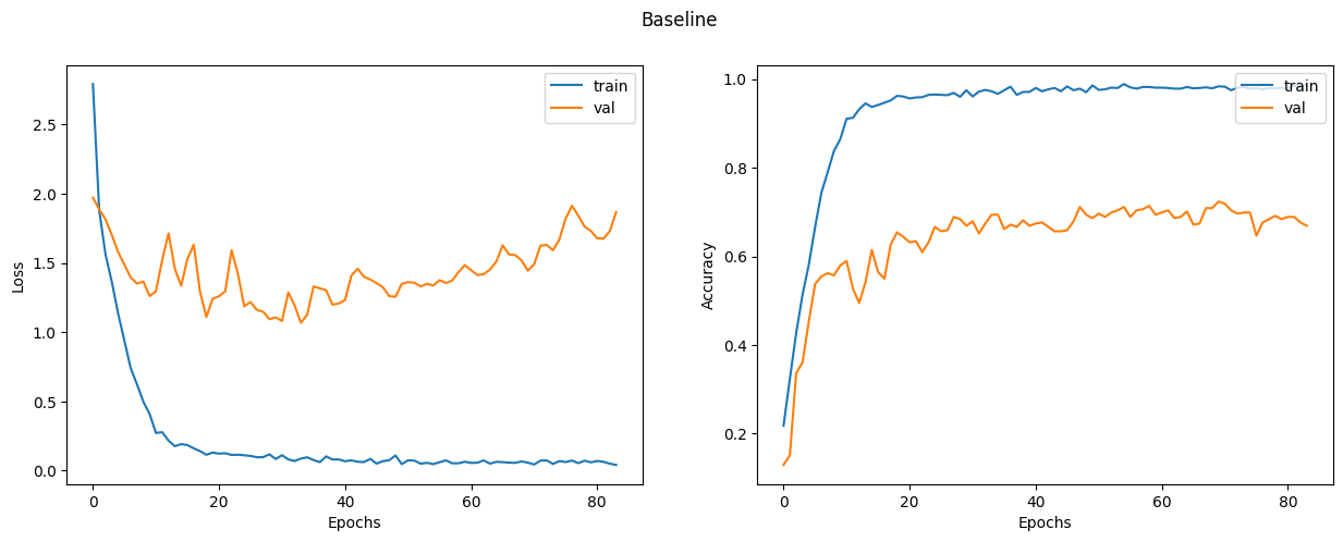
Now we evaluate the baseline model on the test data split.
_, test_accuracy = baseline_model.evaluate(x=x_test_base, y=test_labels, verbose=0)
print(f"Test accuracy: {round(test_accuracy * 100, 2)}%")
Test accuracy: 73.24%
Examine the baseline model predictions
Let's create new data instances by randomly generating binary word vectors with respect to the word presence probabilities.
def generate_random_instances(num_instances):
    token_probability = x_train_base.mean(axis=0)
    instances = []
    for _ in range(num_instances):
        probabilities = np.random.uniform(size=len(token_probability))
        instance = (probabilities <= token_probability).astype(int)
        instances.append(instance)

    return np.array(instances)


def display_class_probabilities(probabilities):
    for instance_idx, probs in enumerate(probabilities):
        print(f"Instance {instance_idx + 1}:")
        for class_idx, prob in enumerate(probs):
            print(f"- {class_values[class_idx]}: {round(prob * 100, 2)}%")
Now we show the baseline model predictions given these randomly generated instances.
new_instances = generate_random_instances(num_classes)
logits = baseline_model.predict(new_instances)
probabilities = ops.convert_to_numpy(
    keras.activations.softmax(ops.convert_to_tensor(logits))
)
display_class_probabilities(probabilities)
1/1 ━━━━━━━━━━━━━━━━━━━━ 0s 120ms/step

Instance 1:
- Case_Based: 0.0%
- Genetic_Algorithms: 99.8499984741211%
- Neural_Networks: 0.09000000357627869%
- Probabilistic_Methods: 0.019999999552965164%
- Reinforcement_Learning: 0.029999999329447746%
- Rule_Learning: 0.009999999776482582%
- Theory: 0.0%
Instance 2:
- Case_Based: 0.47999998927116394%
- Genetic_Algorithms: 0.44999998807907104%
- Neural_Networks: 1.7000000476837158%
- Probabilistic_Methods: 92.27999877929688%
- Reinforcement_Learning: 0.10999999940395355%
- Rule_Learning: 1.149999976158142%
- Theory: 3.8399999141693115%
Instance 3:
- Case_Based: 25.6299991607666%
- Genetic_Algorithms: 0.9200000166893005%
- Neural_Networks: 29.25%
- Probabilistic_Methods: 13.300000190734863%
- Reinforcement_Learning: 1.4800000190734863%
- Rule_Learning: 17.420000076293945%
- Theory: 11.989999771118164%
Instance 4:
- Case_Based: 0.009999999776482582%
- Genetic_Algorithms: 98.80999755859375%
- Neural_Networks: 1.0199999809265137%
- Probabilistic_Methods: 0.029999999329447746%
- Reinforcement_Learning: 0.029999999329447746%
- Rule_Learning: 0.07000000029802322%
- Theory: 0.029999999329447746%
Instance 5:
- Case_Based: 10.199999809265137%
- Genetic_Algorithms: 70.12000274658203%
- Neural_Networks: 6.730000019073486%
- Probabilistic_Methods: 3.9100000858306885%
- Reinforcement_Learning: 3.0399999618530273%
- Rule_Learning: 2.2300000190734863%
- Theory: 3.759999990463257%
Instance 6:
- Case_Based: 50.04999923706055%
- Genetic_Algorithms: 1.2400000095367432%
- Neural_Networks: 5.019999980926514%
- Probabilistic_Methods: 39.45000076293945%
- Reinforcement_Learning: 0.05000000074505806%
- Rule_Learning: 0.23000000417232513%
- Theory: 3.9600000381469727%
Instance 7:
- Case_Based: 0.029999999329447746%
- Genetic_Algorithms: 0.0%
- Neural_Networks: 99.81999969482422%
- Probabilistic_Methods: 0.14000000059604645%
- Reinforcement_Learning: 0.0%
- Rule_Learning: 0.0%
- Theory: 0.0%
Build a Graph Neural Network Model
Prepare the data for the graph model
Preparing and loading the graphs data into the model for training is the most challenging part in GNN models, which is addressed in different ways by the specialised libraries. In this example, we show a simple approach for preparing and using graph data that is suitable if your dataset consists of a single graph that fits entirely in memory.
The graph data is represented by the graph_info tuple, which consists of the following
three elements:
node_features: This is a[num_nodes, num_features]NumPy array that includes the node features. In this dataset, the nodes are the papers, and thenode_featuresare the word-presence binary vectors of each paper.edges: This is[num_edges, num_edges]NumPy array representing a sparse adjacency matrix of the links between the nodes. In this example, the links are the citations between the papers.edge_weights(optional): This is a[num_edges]NumPy array that includes the edge weights, which quantify the relationships between nodes in the graph. In this example, there are no weights for the paper citations.
# Create an edges array (sparse adjacency matrix) of shape [2, num_edges].
edges = citations[["source", "target"]].to_numpy().T
# Create an edge weights array of ones.
edge_weights = ops.ones(shape=edges.shape[1])
# Create a node features array of shape [num_nodes, num_features].
node_features = ops.cast(
    papers.sort_values("paper_id")[feature_names].to_numpy(), dtype="float32"
)
# Create graph info tuple with node_features, edges, and edge_weights.
graph_info = (node_features, edges, edge_weights)

print("Edges shape:", edges.shape)
print("Nodes shape:", node_features.shape)
Edges shape:

 (2, 5429)
Nodes shape: (2708, 1433)
Implement a graph convolution layer
We implement the graph convolution module as a custom Keras 3 Layer. Our GraphConvLayer is designed to be backend-agnostic, utilizing keras.ops to perform the following three steps:
- Prepare: The input node representations are processed using a Feed-Forward Network (FFN) to produce a message. This is achieved by gathering neighbor representations using ops.take and transforming them through the ffn_prepare block. If edge_weights are provided, they are scaled using ops.expand_dims to ensure correct broadcasting during message transformation
- Aggregate: The messages of the neighbors for each node are aggregated using a permutation-invariant pooling operation. In this Keras 3 implementation, we utilize ops.segment_sum, ops.segment_mean, or ops.segment_max (replacing the legacy tf.math.unsorted_segment APIs). These operations efficiently aggregate neighbor information into a single message for each target node based on the graph's edge indices.
- Update: The
node_repesentationsandaggregated_messages—both of shape[num_nodes, representation_dim]— are combined and processed to produce the new state of the node representations (node embeddings). Ifcombination_typeisgru, thenode_repesentationsandaggregated_messagesare stacked to create a sequence, then processed by a GRU layer. Otherwise, thenode_repesentationsandaggregated_messagesare added or concatenated, then processed using a FFN.
The technique implemented use ideas from Graph Convolutional Networks, GraphSage, Graph Isomorphism Network, Simple Graph Networks, and Gated Graph Sequence Neural Networks. Two other key techniques that are not covered are Graph Attention Networks and Message Passing Neural Networks.
def create_gru(hidden_units, dropout_rate):
    inputs = layers.Input(shape=(2, hidden_units[0]))
    x = inputs
    for units in hidden_units:
        x = layers.GRU(
            units=units,
            activation="tanh",
            recurrent_activation="sigmoid",
            return_sequences=True,
            dropout=dropout_rate,
        )(x)
    return keras.Model(inputs=inputs, outputs=x)


class GraphConvLayer(layers.Layer):
    def __init__(
        self,
        hidden_units,
        dropout_rate=0.2,
        aggregation_type="mean",
        combination_type="concat",
        normalize=False,
        **kwargs,
    ):
        super().__init__(**kwargs)
        self.aggregation_type = aggregation_type
        self.combination_type = combination_type
        self.normalize = normalize

        self.ffn_prepare = create_ffn(hidden_units, dropout_rate)
        self.update_fn = (
            create_gru(hidden_units, dropout_rate)
            if combination_type == "gru"
            else create_ffn(hidden_units, dropout_rate)
        )

    def prepare(self, node_representations, weights=None, training=None):
        messages = self.ffn_prepare(node_representations, training=training)
        if weights is not None:
            messages = messages * ops.expand_dims(weights, -1)
        return messages

    def aggregate(self, node_indices, neighbour_messages, node_representations):
        num_nodes = ops.shape(node_representations)[0]
        if self.aggregation_type == "sum":
            return ops.segment_sum(
                neighbour_messages, node_indices, num_segments=num_nodes
            )
        elif self.aggregation_type == "mean":
            return ops.segment_mean(
                neighbour_messages, node_indices, num_segments=num_nodes
            )
        elif self.aggregation_type == "max":
            return ops.segment_max(
                neighbour_messages, node_indices, num_segments=num_nodes
            )
        else:
            raise ValueError(f"Invalid aggregation type: {self.aggregation_type}")

    def update(self, node_representations, aggregated_messages, training=None):
        if self.combination_type == "gru":
            h = ops.stack([node_representations, aggregated_messages], axis=1)
        elif self.combination_type == "concat":
            h = ops.concatenate([node_representations, aggregated_messages], axis=-1)
        elif self.combination_type == "add":
            h = node_representations + aggregated_messages
        else:
            raise ValueError(f"Invalid combination type: {self.combination_type}")

        node_embeddings = self.update_fn(h, training=training)

        if self.combination_type == "gru":
            node_embeddings = ops.unstack(node_embeddings, axis=1)[-1]

        if self.normalize:
            node_embeddings = ops.normalize(node_embeddings, axis=-1, order=2)
        return node_embeddings

    def call(self, inputs, training=None):
        node_representations, edges, edge_weights = inputs
        node_indices, neighbour_indices = edges[0], edges[1]
        neighbour_representations = ops.take(
            node_representations, neighbour_indices, axis=0
        )

        neighbour_messages = self.prepare(
            neighbour_representations, edge_weights, training=training
        )
        aggregated_messages = self.aggregate(
            node_indices, neighbour_messages, node_representations
        )
        return self.update(node_representations, aggregated_messages, training=training)
Implement a graph neural network node classifier
The GNN classification model follows the Design Space for Graph Neural Networks approach, as follows:
Graph Augmentation & Stability: In the init method, the model optionally adds self-loops to the edge list. This ensures each node preserves its own identity during message passing. We also implement Edge Weight Normalization (Global or Per-node). Per-node normalization calculates the degree of each node using ops.segment_sum and scales incoming messages, which is critical for preventing gradient explosion in large or dense graphs. Preprocessing: A Feed-Forward Network (FFN) is applied to the raw node features to generate the initial latent representations. Graph Convolutions with Skip Connections: The model applies multiple GraphConvLayer blocks. To mitigate the risk of "over-smoothing" (where node embeddings become indistinguishable after several hops), we implement Residual (Skip) Connections, adding the input of the convolution back to its output. Post-processing: A final FFN processes the node embeddings to refine the features before classification. Output Logic: The final layer is a Dense layer that produces logits for each class. Note on Data Handling: Unlike standard models where all data is passed as input, this model stores the global graph structure (node_features and edges) as internal tensors converted via ops.convert_to_tensor. The model's call() method accepts a batch of node indices rather than the full graph. It uses ops.take to efficiently retrieve the specific embeddings for the requested indices, allowing for efficient mini-batch training on a single large graph.
class GNNNodeClassifier(keras.Model):
    def __init__(
        self,
        graph_info,
        num_classes,
        hidden_units,
        aggregation_type="sum",
        combination_type="concat",
        dropout_rate=0.5,
        normalize=True,
        add_self_loops=True,
        edge_weight_normalization="per_node",  # "none" | "global" | "per_node"
        **kwargs,
    ):
        super().__init__(**kwargs)

        node_features, edges, edge_weights = graph_info
        num_nodes = node_features.shape[0]

        self.node_features = ops.convert_to_tensor(node_features, dtype="float32")

        if add_self_loops:
            self_loops = np.stack(
                [np.arange(num_nodes), np.arange(num_nodes)], axis=0
            ).astype("int32")
            edges = np.concatenate([edges, self_loops], axis=1)

        self.edges = ops.convert_to_tensor(edges, dtype="int32")

        num_edges = edges.shape[1]
        if edge_weights is None:
            edge_weights = ops.ones(shape=(num_edges,), dtype="float32")
        else:
            edge_weights = ops.convert_to_tensor(edge_weights, dtype="float32")
            if add_self_loops:
                loop_weights = ops.ones(shape=(num_nodes,), dtype="float32")
                edge_weights = ops.concatenate([edge_weights, loop_weights], axis=0)

        if edge_weight_normalization == "global":
            edge_weights = edge_weights / (ops.sum(edge_weights) + 1e-7)
        elif edge_weight_normalization == "per_node":
            node_indices = self.edges[0]
            deg = ops.segment_sum(edge_weights, node_indices, num_segments=num_nodes)
            deg = ops.maximum(deg, 1.0)
            edge_weights = edge_weights / ops.take(deg, node_indices, axis=0)
        elif edge_weight_normalization == "none":
            pass
        else:
            raise ValueError(
                "edge_weight_normalization must be 'none', 'global', or 'per_node'."
            )

        self.edge_weights = edge_weights

        self.preprocess = create_ffn(hidden_units, dropout_rate, name="preprocess")
        self.conv1 = GraphConvLayer(
            hidden_units,
            dropout_rate=dropout_rate,
            aggregation_type=aggregation_type,
            combination_type=combination_type,
            normalize=normalize,
            name="graph_conv1",
        )
        self.conv2 = GraphConvLayer(
            hidden_units,
            dropout_rate=dropout_rate,
            aggregation_type=aggregation_type,
            combination_type=combination_type,
            normalize=normalize,
            name="graph_conv2",
        )
        self.postprocess = create_ffn(hidden_units, dropout_rate, name="postprocess")
        self.compute_logits = layers.Dense(num_classes, name="logits")

    def call(self, input_node_indices, training=None):
        x = self.preprocess(self.node_features, training=training)

        x1 = self.conv1((x, self.edges, self.edge_weights), training=training)
        x = x + x1

        x2 = self.conv2((x, self.edges, self.edge_weights), training=training)
        x = x + x2

        x = self.postprocess(x, training=training)
        node_embeddings = ops.take(x, input_node_indices, axis=0)
        return self.compute_logits(node_embeddings)
Let's test instantiating and calling the GNN model.
Notice that if you provide N node indices, the output will be a tensor of shape [N, num_classes],
regardless of the size of the graph.
gnn_model = GNNNodeClassifier(
    graph_info=graph_info,
    num_classes=num_classes,
    hidden_units=[32, 32],
    aggregation_type="sum",
    combination_type="concat",
    dropout_rate=0.5,
    normalize=True,
    add_self_loops=True,
    edge_weight_normalization="per_node",
    name="gnn_model",
)

print("GNN output shape:", gnn_model(ops.convert_to_tensor([0, 1, 2], dtype="int32")))

gnn_model.summary()
GNN output shape: tf.Tensor(
[[ 0.12753698 -0.03277592  0.12849751 -0.12325159 -0.03344828 -0.00571804
   0.07434124]
 [ 0.06960323  0.06341869 -0.03549282  0.00485269 -0.03028604  0.07213619
  -0.0552844 ]
 [-0.10136008  0.1263252  -0.07481521  0.05478853  0.01184586  0.03908347
  -0.00210544]], shape=(3, 7), dtype=float32)
Model: "gnn_model"
┏━━━━━━━━━━━━━━━━━━━━━━━━━━━━━━━━━┳━━━━━━━━━━━━━━━━━━━━━━━━┳━━━━━━━━━━━━━━━┓
┃ Layer (type)                    ┃ Output Shape           ┃       Param # ┃
┡━━━━━━━━━━━━━━━━━━━━━━━━━━━━━━━━━╇━━━━━━━━━━━━━━━━━━━━━━━━╇━━━━━━━━━━━━━━━┩
│ preprocess (Sequential)         │ (2708, 32)             │        52,804 │
├─────────────────────────────────┼────────────────────────┼───────────────┤
│ graph_conv1 (GraphConvLayer)    │ ?                      │         5,888 │
├─────────────────────────────────┼────────────────────────┼───────────────┤
│ graph_conv2 (GraphConvLayer)    │ ?                      │         5,888 │
├─────────────────────────────────┼────────────────────────┼───────────────┤
│ postprocess (Sequential)        │ (2708, 32)             │         2,368 │
├─────────────────────────────────┼────────────────────────┼───────────────┤
│ logits (Dense)                  │ (3, 7)                 │           231 │
└─────────────────────────────────┴────────────────────────┴───────────────┘
Total params: 67,179 (262.42 KB)
Trainable params: 63,481 (247.97 KB)
Non-trainable params: 3,698 (14.45 KB)
Train the GNN model
Note that we use the standard supervised cross-entropy loss to train the model. However, we can add another self-supervised loss term for the generated node embeddings that makes sure that neighbouring nodes in graph have similar representations, while faraway nodes have dissimilar representations.
gnn_history = run_experiment(
    gnn_model,
    train_indices,
    train_labels,
    val_indices,
    val_labels,
)
Epoch 1/300

6/6 - 3s - 542ms/step - acc: 0.1589 - loss: 2.2321 - val_acc: 0.3035 - val_loss: 1.8884

Epoch 2/300

6/6 - 0s - 46ms/step - acc: 0.2624 - loss: 1.9686 - val_acc: 0.3035 - val_loss: 1.8717

Epoch 3/300

6/6 - 0s - 46ms/step - acc: 0.2897 - loss: 1.8916 - val_acc: 0.3035 - val_loss: 1.8694

Epoch 4/300

6/6 - 0s - 46ms/step - acc: 0.2868 - loss: 1.8492 - val_acc: 0.3035 - val_loss: 1.8688

Epoch 5/300

6/6 - 0s - 47ms/step - acc: 0.2882 - loss: 1.8489 - val_acc: 0.3035 - val_loss: 1.8648

Epoch 6/300

6/6 - 0s - 47ms/step - acc: 0.2949 - loss: 1.8408 - val_acc: 0.3035 - val_loss: 1.8564

Epoch 7/300

6/6 - 0s - 47ms/step - acc: 0.2979 - loss: 1.8190 - val_acc: 0.3035 - val_loss: 1.8500

Epoch 8/300

6/6 - 0s - 47ms/step - acc: 0.3016 - loss: 1.8054 - val_acc: 0.3060 - val_loss: 1.8437

Epoch 9/300

6/6 - 0s - 47ms/step - acc: 0.3252 - loss: 1.8077 - val_acc: 0.3234 - val_loss: 1.8318

Epoch 10/300

6/6 - 0s - 47ms/step - acc: 0.3282 - loss: 1.7648 - val_acc: 0.3731 - val_loss: 1.8247

Epoch 11/300

6/6 - 0s - 47ms/step - acc: 0.3311 - loss: 1.7490 - val_acc: 0.3682 - val_loss: 1.8271

Epoch 12/300

6/6 - 0s - 48ms/step - acc: 0.3400 - loss: 1.7138 - val_acc: 0.2388 - val_loss: 1.8482

Epoch 13/300

6/6 - 0s - 47ms/step - acc: 0.3622 - loss: 1.6725 - val_acc: 0.2114 - val_loss: 1.8837

Epoch 14/300

6/6 - 0s - 48ms/step - acc: 0.3917 - loss: 1.6194 - val_acc: 0.2438 - val_loss: 1.8811

Epoch 15/300

6/6 - 0s - 47ms/step - acc: 0.4065 - loss: 1.5838 - val_acc: 0.2836 - val_loss: 1.8569

Epoch 16/300

6/6 - 0s - 50ms/step - acc: 0.4287 - loss: 1.5212 - val_acc: 0.3408 - val_loss: 1.7707

Epoch 17/300

6/6 - 0s - 53ms/step - acc: 0.4597 - loss: 1.5125 - val_acc: 0.4005 - val_loss: 1.7040

Epoch 18/300

6/6 - 0s - 53ms/step - acc: 0.4612 - loss: 1.4562 - val_acc: 0.4602 - val_loss: 1.4365

Epoch 19/300

6/6 - 0s - 53ms/step - acc: 0.4937 - loss: 1.3864 - val_acc: 0.4577 - val_loss: 1.5052

Epoch 20/300

6/6 - 0s - 53ms/step - acc: 0.5137 - loss: 1.3652 - val_acc: 0.4378 - val_loss: 1.5751

Epoch 21/300

6/6 - 0s - 53ms/step - acc: 0.5063 - loss: 1.3094 - val_acc: 0.4552 - val_loss: 1.5617

Epoch 22/300

6/6 - 0s - 53ms/step - acc: 0.5344 - loss: 1.3068 - val_acc: 0.4851 - val_loss: 1.5253

Epoch 23/300

6/6 - 0s - 58ms/step - acc: 0.5469 - loss: 1.2459 - val_acc: 0.4751 - val_loss: 1.3819

Epoch 24/300

6/6 - 0s - 55ms/step - acc: 0.5558 - loss: 1.2252 - val_acc: 0.6070 - val_loss: 1.0655

Epoch 25/300

6/6 - 0s - 55ms/step - acc: 0.5846 - loss: 1.1600 - val_acc: 0.6592 - val_loss: 1.0230

Epoch 26/300

6/6 - 0s - 54ms/step - acc: 0.5920 - loss: 1.1357 - val_acc: 0.6393 - val_loss: 1.0505

Epoch 27/300

6/6 - 0s - 55ms/step - acc: 0.5735 - loss: 1.1590 - val_acc: 0.6517 - val_loss: 1.0781

Epoch 28/300

6/6 - 0s - 64ms/step - acc: 0.6001 - loss: 1.0819 - val_acc: 0.6567 - val_loss: 1.0271

Epoch 29/300

6/6 - 0s - 61ms/step - acc: 0.6024 - loss: 1.1185 - val_acc: 0.6567 - val_loss: 0.9653

Epoch 30/300

6/6 - 0s - 61ms/step - acc: 0.6349 - loss: 1.0402 - val_acc: 0.6418 - val_loss: 0.9459

Epoch 31/300

6/6 - 0s - 55ms/step - acc: 0.6438 - loss: 1.0170 - val_acc: 0.6692 - val_loss: 0.9221

Epoch 32/300

6/6 - 0s - 53ms/step - acc: 0.6378 - loss: 0.9892 - val_acc: 0.6567 - val_loss: 0.9809

Epoch 33/300

6/6 - 0s - 54ms/step - acc: 0.6401 - loss: 0.9891 - val_acc: 0.6667 - val_loss: 0.9195

Epoch 34/300

6/6 - 0s - 55ms/step - acc: 0.6622 - loss: 0.9481 - val_acc: 0.6866 - val_loss: 0.8954

Epoch 35/300

6/6 - 0s - 54ms/step - acc: 0.6482 - loss: 0.9554 - val_acc: 0.6766 - val_loss: 0.8609

Epoch 36/300

6/6 - 0s - 54ms/step - acc: 0.6681 - loss: 0.9062 - val_acc: 0.6642 - val_loss: 0.8538

Epoch 37/300

6/6 - 0s - 53ms/step - acc: 0.6674 - loss: 0.9389 - val_acc: 0.6965 - val_loss: 0.8263

Epoch 38/300

6/6 - 0s - 54ms/step - acc: 0.6593 - loss: 0.9298 - val_acc: 0.7040 - val_loss: 0.8462

Epoch 39/300

6/6 - 0s - 54ms/step - acc: 0.6807 - loss: 0.8722 - val_acc: 0.6866 - val_loss: 0.8878

Epoch 40/300

6/6 - 0s - 54ms/step - acc: 0.6755 - loss: 0.8960 - val_acc: 0.6766 - val_loss: 0.8864

Epoch 41/300

6/6 - 0s - 54ms/step - acc: 0.6940 - loss: 0.8764 - val_acc: 0.6667 - val_loss: 0.8792

Epoch 42/300

6/6 - 0s - 56ms/step - acc: 0.6689 - loss: 0.9039 - val_acc: 0.6841 - val_loss: 0.8488

Epoch 43/300

6/6 - 0s - 53ms/step - acc: 0.6733 - loss: 0.8917 - val_acc: 0.6542 - val_loss: 0.8978

Epoch 44/300

6/6 - 0s - 55ms/step - acc: 0.6911 - loss: 0.8295 - val_acc: 0.6244 - val_loss: 1.0138

Epoch 45/300

6/6 - 0s - 53ms/step - acc: 0.7036 - loss: 0.8178 - val_acc: 0.6791 - val_loss: 0.9167

Epoch 46/300

6/6 - 0s - 54ms/step - acc: 0.7169 - loss: 0.8118 - val_acc: 0.6766 - val_loss: 0.9275

Epoch 47/300

6/6 - 0s - 53ms/step - acc: 0.7147 - loss: 0.8344 - val_acc: 0.6667 - val_loss: 0.8843

Epoch 48/300

6/6 - 0s - 54ms/step - acc: 0.7236 - loss: 0.8182 - val_acc: 0.6841 - val_loss: 0.8684

Epoch 49/300

6/6 - 0s - 54ms/step - acc: 0.7214 - loss: 0.7890 - val_acc: 0.6866 - val_loss: 0.8972

Epoch 50/300

6/6 - 0s - 54ms/step - acc: 0.6999 - loss: 0.8039 - val_acc: 0.6965 - val_loss: 0.8798

Epoch 51/300

6/6 - 0s - 54ms/step - acc: 0.7029 - loss: 0.8262 - val_acc: 0.6841 - val_loss: 0.8527

Epoch 52/300

6/6 - 0s - 55ms/step - acc: 0.7206 - loss: 0.7723 - val_acc: 0.7040 - val_loss: 0.7963

Epoch 53/300

6/6 - 0s - 54ms/step - acc: 0.7280 - loss: 0.7551 - val_acc: 0.7214 - val_loss: 0.7786

Epoch 54/300

6/6 - 0s - 54ms/step - acc: 0.7243 - loss: 0.7633 - val_acc: 0.7313 - val_loss: 0.8068

Epoch 55/300

6/6 - 0s - 54ms/step - acc: 0.7354 - loss: 0.7493 - val_acc: 0.7214 - val_loss: 0.8281

Epoch 56/300

6/6 - 0s - 54ms/step - acc: 0.7398 - loss: 0.7262 - val_acc: 0.7040 - val_loss: 0.8875

Epoch 57/300

6/6 - 0s - 55ms/step - acc: 0.7324 - loss: 0.7632 - val_acc: 0.6617 - val_loss: 1.0027

Epoch 58/300

6/6 - 0s - 55ms/step - acc: 0.7450 - loss: 0.7710 - val_acc: 0.6841 - val_loss: 0.9042

Epoch 59/300

6/6 - 0s - 53ms/step - acc: 0.7472 - loss: 0.7079 - val_acc: 0.7139 - val_loss: 0.8433

Epoch 60/300

6/6 - 0s - 55ms/step - acc: 0.7310 - loss: 0.7903 - val_acc: 0.7363 - val_loss: 0.8285

Epoch 61/300

6/6 - 0s - 54ms/step - acc: 0.7561 - loss: 0.6845 - val_acc: 0.7239 - val_loss: 0.8113

Epoch 62/300

6/6 - 0s - 54ms/step - acc: 0.7435 - loss: 0.7162 - val_acc: 0.7139 - val_loss: 0.8309

Epoch 63/300

6/6 - 0s - 54ms/step - acc: 0.7458 - loss: 0.7156 - val_acc: 0.7338 - val_loss: 0.7957

Epoch 64/300

6/6 - 0s - 55ms/step - acc: 0.7428 - loss: 0.6854 - val_acc: 0.7313 - val_loss: 0.7933

Epoch 65/300

6/6 - 0s - 57ms/step - acc: 0.7295 - loss: 0.7536 - val_acc: 0.7413 - val_loss: 0.7843

Epoch 66/300

6/6 - 0s - 54ms/step - acc: 0.7494 - loss: 0.7285 - val_acc: 0.7139 - val_loss: 0.7730

Epoch 67/300

6/6 - 0s - 55ms/step - acc: 0.7620 - loss: 0.6678 - val_acc: 0.7289 - val_loss: 0.7617

Epoch 68/300

6/6 - 0s - 53ms/step - acc: 0.7472 - loss: 0.6998 - val_acc: 0.7363 - val_loss: 0.7817

Epoch 69/300

6/6 - 0s - 54ms/step - acc: 0.7458 - loss: 0.7076 - val_acc: 0.7438 - val_loss: 0.7878

Epoch 70/300

6/6 - 0s - 54ms/step - acc: 0.7679 - loss: 0.6606 - val_acc: 0.7537 - val_loss: 0.7586

Epoch 71/300

6/6 - 0s - 54ms/step - acc: 0.7679 - loss: 0.6766 - val_acc: 0.7313 - val_loss: 0.8017

Epoch 72/300

6/6 - 0s - 54ms/step - acc: 0.7709 - loss: 0.6723 - val_acc: 0.7562 - val_loss: 0.7683

Epoch 73/300

6/6 - 0s - 56ms/step - acc: 0.7450 - loss: 0.7229 - val_acc: 0.7438 - val_loss: 0.7506

Epoch 74/300

6/6 - 0s - 54ms/step - acc: 0.7768 - loss: 0.6576 - val_acc: 0.7537 - val_loss: 0.7641

Epoch 75/300

6/6 - 0s - 54ms/step - acc: 0.7746 - loss: 0.6791 - val_acc: 0.7488 - val_loss: 0.7580

Epoch 76/300

6/6 - 0s - 55ms/step - acc: 0.7842 - loss: 0.6325 - val_acc: 0.7687 - val_loss: 0.7615

Epoch 77/300

6/6 - 0s - 54ms/step - acc: 0.7576 - loss: 0.7195 - val_acc: 0.7761 - val_loss: 0.7805

Epoch 78/300

6/6 - 0s - 54ms/step - acc: 0.7701 - loss: 0.6787 - val_acc: 0.7836 - val_loss: 0.7738

Epoch 79/300

6/6 - 0s - 54ms/step - acc: 0.7805 - loss: 0.6446 - val_acc: 0.7836 - val_loss: 0.7537

Epoch 80/300

6/6 - 0s - 54ms/step - acc: 0.7886 - loss: 0.6125 - val_acc: 0.7562 - val_loss: 0.7870

Epoch 81/300

6/6 - 0s - 54ms/step - acc: 0.7842 - loss: 0.6550 - val_acc: 0.7637 - val_loss: 0.7847

Epoch 82/300

6/6 - 0s - 54ms/step - acc: 0.7886 - loss: 0.5922 - val_acc: 0.7637 - val_loss: 0.8269

Epoch 83/300

6/6 - 0s - 54ms/step - acc: 0.7687 - loss: 0.6950 - val_acc: 0.7512 - val_loss: 0.8055

Epoch 84/300

6/6 - 0s - 55ms/step - acc: 0.7931 - loss: 0.6359 - val_acc: 0.7811 - val_loss: 0.7970

Epoch 85/300

6/6 - 0s - 55ms/step - acc: 0.7834 - loss: 0.6204 - val_acc: 0.7811 - val_loss: 0.7874

Epoch 86/300

6/6 - 0s - 55ms/step - acc: 0.8041 - loss: 0.5851 - val_acc: 0.7786 - val_loss: 0.7754

Epoch 87/300

6/6 - 0s - 54ms/step - acc: 0.7960 - loss: 0.6140 - val_acc: 0.7761 - val_loss: 0.7664

Epoch 88/300

6/6 - 0s - 55ms/step - acc: 0.7797 - loss: 0.7035 - val_acc: 0.8010 - val_loss: 0.7242

Epoch 89/300

6/6 - 0s - 54ms/step - acc: 0.8174 - loss: 0.5918 - val_acc: 0.7662 - val_loss: 0.7590

Epoch 90/300

6/6 - 0s - 55ms/step - acc: 0.7761 - loss: 0.6620 - val_acc: 0.7886 - val_loss: 0.7376

Epoch 91/300

6/6 - 0s - 55ms/step - acc: 0.7834 - loss: 0.6606 - val_acc: 0.7960 - val_loss: 0.7426

Epoch 92/300

6/6 - 0s - 59ms/step - acc: 0.8071 - loss: 0.5690 - val_acc: 0.7985 - val_loss: 0.7654

Epoch 93/300

6/6 - 0s - 54ms/step - acc: 0.7960 - loss: 0.5890 - val_acc: 0.7960 - val_loss: 0.7775

Epoch 94/300

6/6 - 0s - 55ms/step - acc: 0.8226 - loss: 0.5532 - val_acc: 0.7985 - val_loss: 0.7774

Epoch 95/300

6/6 - 0s - 53ms/step - acc: 0.8034 - loss: 0.6015 - val_acc: 0.7985 - val_loss: 0.7890

Epoch 96/300

6/6 - 0s - 58ms/step - acc: 0.7945 - loss: 0.6226 - val_acc: 0.7985 - val_loss: 0.7568

Epoch 97/300

6/6 - 0s - 55ms/step - acc: 0.8182 - loss: 0.5411 - val_acc: 0.8010 - val_loss: 0.7475

Epoch 98/300

6/6 - 0s - 55ms/step - acc: 0.8271 - loss: 0.5360 - val_acc: 0.8109 - val_loss: 0.7650

Epoch 99/300

6/6 - 0s - 54ms/step - acc: 0.8056 - loss: 0.5896 - val_acc: 0.7910 - val_loss: 0.7855

Epoch 100/300

6/6 - 0s - 55ms/step - acc: 0.8123 - loss: 0.5659 - val_acc: 0.7761 - val_loss: 0.8070

Epoch 101/300

6/6 - 0s - 54ms/step - acc: 0.8004 - loss: 0.5891 - val_acc: 0.7886 - val_loss: 0.7861

Epoch 102/300

6/6 - 0s - 54ms/step - acc: 0.8115 - loss: 0.5753 - val_acc: 0.7910 - val_loss: 0.7720

Epoch 103/300

6/6 - 0s - 56ms/step - acc: 0.7908 - loss: 0.6017 - val_acc: 0.7861 - val_loss: 0.7501

Epoch 104/300

6/6 - 0s - 55ms/step - acc: 0.8160 - loss: 0.5577 - val_acc: 0.7836 - val_loss: 0.7951

Epoch 105/300

6/6 - 0s - 54ms/step - acc: 0.8226 - loss: 0.5284 - val_acc: 0.7985 - val_loss: 0.7921

Epoch 106/300

6/6 - 0s - 55ms/step - acc: 0.8263 - loss: 0.5539 - val_acc: 0.7886 - val_loss: 0.7923

Epoch 107/300

6/6 - 0s - 54ms/step - acc: 0.8389 - loss: 0.5190 - val_acc: 0.7985 - val_loss: 0.7819

Epoch 108/300

6/6 - 0s - 54ms/step - acc: 0.8108 - loss: 0.5686 - val_acc: 0.7861 - val_loss: 0.7826

Epoch 109/300

6/6 - 0s - 55ms/step - acc: 0.8367 - loss: 0.5480 - val_acc: 0.7910 - val_loss: 0.7910

Epoch 110/300

6/6 - 0s - 55ms/step - acc: 0.8307 - loss: 0.5351 - val_acc: 0.7761 - val_loss: 0.8031

Epoch 111/300

6/6 - 0s - 55ms/step - acc: 0.8219 - loss: 0.5524 - val_acc: 0.7861 - val_loss: 0.8318

Epoch 112/300

6/6 - 0s - 55ms/step - acc: 0.8137 - loss: 0.5515 - val_acc: 0.7786 - val_loss: 0.8254

Epoch 113/300

6/6 - 0s - 55ms/step - acc: 0.8241 - loss: 0.5554 - val_acc: 0.7811 - val_loss: 0.8054

Epoch 114/300

6/6 - 0s - 55ms/step - acc: 0.8344 - loss: 0.5209 - val_acc: 0.7836 - val_loss: 0.7945

Epoch 115/300

6/6 - 0s - 55ms/step - acc: 0.8278 - loss: 0.5520 - val_acc: 0.7662 - val_loss: 0.7817

Epoch 116/300

6/6 - 0s - 77ms/step - acc: 0.8344 - loss: 0.5178 - val_acc: 0.7562 - val_loss: 0.8063

Epoch 117/300

6/6 - 0s - 55ms/step - acc: 0.8322 - loss: 0.5529 - val_acc: 0.7761 - val_loss: 0.8042

Epoch 118/300

6/6 - 0s - 55ms/step - acc: 0.8130 - loss: 0.5684 - val_acc: 0.7861 - val_loss: 0.7532

Epoch 119/300

6/6 - 0s - 55ms/step - acc: 0.8152 - loss: 0.5575 - val_acc: 0.7886 - val_loss: 0.7423

Epoch 120/300

6/6 - 0s - 55ms/step - acc: 0.8241 - loss: 0.5438 - val_acc: 0.7836 - val_loss: 0.7407

Epoch 121/300

6/6 - 0s - 56ms/step - acc: 0.8404 - loss: 0.5148 - val_acc: 0.8060 - val_loss: 0.7538

Epoch 122/300

6/6 - 0s - 55ms/step - acc: 0.8204 - loss: 0.5559 - val_acc: 0.8134 - val_loss: 0.7666

Epoch 123/300

6/6 - 0s - 55ms/step - acc: 0.8293 - loss: 0.5143 - val_acc: 0.8035 - val_loss: 0.7436

Epoch 124/300

6/6 - 0s - 55ms/step - acc: 0.8300 - loss: 0.5152 - val_acc: 0.7836 - val_loss: 0.7740

Epoch 125/300

6/6 - 0s - 55ms/step - acc: 0.8389 - loss: 0.5313 - val_acc: 0.7861 - val_loss: 0.7665

Epoch 126/300

6/6 - 0s - 55ms/step - acc: 0.8293 - loss: 0.5244 - val_acc: 0.7935 - val_loss: 0.7501

Epoch 127/300

6/6 - 0s - 55ms/step - acc: 0.8322 - loss: 0.5531 - val_acc: 0.8085 - val_loss: 0.7636

Epoch 128/300

6/6 - 0s - 54ms/step - acc: 0.8293 - loss: 0.5271 - val_acc: 0.7935 - val_loss: 0.7807

Epoch 129/300

6/6 - 0s - 65ms/step - acc: 0.8559 - loss: 0.4785 - val_acc: 0.8010 - val_loss: 0.7853

Epoch 130/300

6/6 - 0s - 55ms/step - acc: 0.8470 - loss: 0.5245 - val_acc: 0.7910 - val_loss: 0.7929

Epoch 131/300

6/6 - 0s - 56ms/step - acc: 0.8433 - loss: 0.5023 - val_acc: 0.7886 - val_loss: 0.7717

Epoch 132/300

6/6 - 0s - 55ms/step - acc: 0.8426 - loss: 0.5015 - val_acc: 0.7836 - val_loss: 0.7627

Epoch 133/300

6/6 - 0s - 56ms/step - acc: 0.8418 - loss: 0.5061 - val_acc: 0.7960 - val_loss: 0.8012

Epoch 134/300

6/6 - 0s - 55ms/step - acc: 0.8433 - loss: 0.5127 - val_acc: 0.8035 - val_loss: 0.8005

Epoch 135/300

6/6 - 0s - 56ms/step - acc: 0.8500 - loss: 0.4648 - val_acc: 0.7960 - val_loss: 0.7991

Epoch 136/300

6/6 - 0s - 55ms/step - acc: 0.8470 - loss: 0.5142 - val_acc: 0.7886 - val_loss: 0.8174

Epoch 137/300

6/6 - 0s - 55ms/step - acc: 0.8374 - loss: 0.5044 - val_acc: 0.7985 - val_loss: 0.8255

Epoch 138/300

6/6 - 0s - 56ms/step - acc: 0.8596 - loss: 0.4605 - val_acc: 0.7985 - val_loss: 0.7835
Let's plot the learning curves
display_learning_curves(gnn_history, title="GNN")
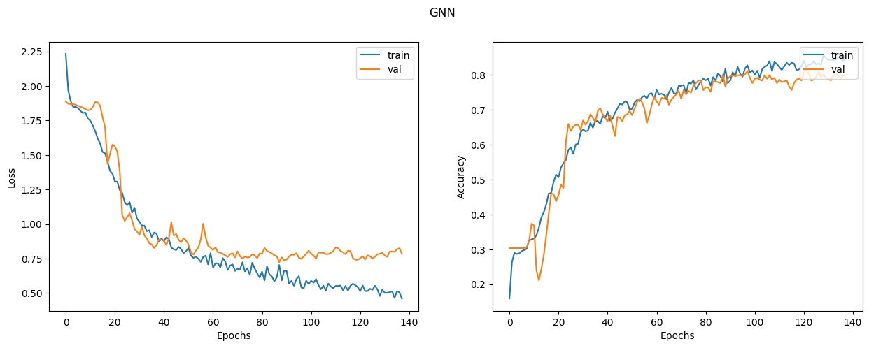
Now we evaluate the GNN model on the test data split. The results may vary depending on the training sample, however the GNN model always outperforms the baseline model in terms of the test accuracy.
x_test = test_indices
_, test_accuracy = gnn_model.evaluate(x=test_indices, y=test_labels, verbose=0)
print(f"Test accuracy: {round(test_accuracy * 100, 2)}%")
Test accuracy: 80.27%
Examine the GNN model predictions
Let's add the new instances as nodes to the node_features, and generate links
(citations) to existing nodes.
# First we add the N new_instances as nodes to the graph
# by appending the new_instance to node_features.
num_nodes = int(gnn_model.node_features.shape[0])

new_instances = new_instances.astype("float32")

new_node_features = np.concatenate(
    [ops.convert_to_numpy(gnn_model.node_features), new_instances], axis=0
).astype("float32")

new_node_indices = np.arange(num_nodes, num_nodes + num_classes, dtype="int32")

new_citations = []
for subject_idx, group in papers.groupby("subject"):
    subject_papers = group.paper_id.to_numpy()

    selected_paper_indices1 = np.random.choice(subject_papers, 5, replace=False)

    selected_paper_indices2 = np.random.choice(
        papers.paper_id.to_numpy(), 2, replace=False
    )

    selected_paper_indices = np.concatenate(
        [selected_paper_indices1, selected_paper_indices2], axis=0
    )

    # Create edges between a citing paper idx and the selected cited papers.
    citing_paper_idx = int(new_node_indices[int(subject_idx)])
    for cited_paper_idx in selected_paper_indices:
        new_citations.append([citing_paper_idx, int(cited_paper_idx)])

new_citations = np.array(new_citations, dtype="int32").T
new_edges = np.concatenate(
    [ops.convert_to_numpy(gnn_model.edges), new_citations], axis=1
).astype("int32")

# Optional but recommended for consistency..add self-loops for the NEW nodes too.
new_self_loops = np.stack([new_node_indices, new_node_indices], axis=0).astype("int32")
new_edges = np.concatenate([new_edges, new_self_loops], axis=1)
Now let's update the node_features and the edges in the GNN model.
print("Original node_features shape:", gnn_model.node_features.shape)
print("Original edges shape:", gnn_model.edges.shape)

# Update model graph
gnn_model.node_features = ops.convert_to_tensor(new_node_features, dtype="float32")
gnn_model.edges = ops.convert_to_tensor(new_edges, dtype="int32")
gnn_model.edge_weights = ops.ones(shape=(new_edges.shape[1],), dtype="float32")

print("New node_features shape:", gnn_model.node_features.shape)
print("New edges shape:", gnn_model.edges.shape)

# Predict on the new nodes
logits = gnn_model(
    ops.convert_to_tensor(new_node_indices, dtype="int32"), training=False
)
probabilities = ops.convert_to_numpy(ops.softmax(logits))
display_class_probabilities(probabilities)
Original node_features shape: (2708, 1433)
Original edges shape: (2, 8137)
New node_features shape: (2715, 1433)
New edges shape: (2, 8193)
Instance 1:
- Case_Based: 7.650000095367432%
- Genetic_Algorithms: 9.75%
- Neural_Networks: 3.940000057220459%
- Probabilistic_Methods: 52.869998931884766%
- Reinforcement_Learning: 1.649999976158142%
- Rule_Learning: 12.670000076293945%
- Theory: 11.460000038146973%
Instance 2:
- Case_Based: 1.690000057220459%
- Genetic_Algorithms: 74.70999908447266%
- Neural_Networks: 2.5899999141693115%
- Probabilistic_Methods: 7.230000019073486%
- Reinforcement_Learning: 11.630000114440918%
- Rule_Learning: 0.7099999785423279%
- Theory: 1.4299999475479126%
Instance 3:
- Case_Based: 2.640000104904175%
- Genetic_Algorithms: 1.149999976158142%
- Neural_Networks: 63.33000183105469%
- Probabilistic_Methods: 4.079999923706055%
- Reinforcement_Learning: 2.7200000286102295%
- Rule_Learning: 3.430000066757202%
- Theory: 22.649999618530273%
Instance 4:
- Case_Based: 6.809999942779541%
- Genetic_Algorithms: 42.43000030517578%
- Neural_Networks: 3.0399999618530273%
- Probabilistic_Methods: 33.369998931884766%
- Reinforcement_Learning: 5.590000152587891%
- Rule_Learning: 3.9800000190734863%
- Theory: 4.78000020980835%
Instance 5:
- Case_Based: 1.0399999618530273%
- Genetic_Algorithms: 41.72999954223633%
- Neural_Networks: 2.559999942779541%
- Probabilistic_Methods: 0.5%
- Reinforcement_Learning: 53.400001525878906%
- Rule_Learning: 0.12999999523162842%
- Theory: 0.6399999856948853%
Instance 6:
- Case_Based: 76.2300033569336%
- Genetic_Algorithms: 0.6600000262260437%
- Neural_Networks: 2.009999990463257%
- Probabilistic_Methods: 13.069999694824219%
- Reinforcement_Learning: 0.41999998688697815%
- Rule_Learning: 1.8600000143051147%
- Theory: 5.760000228881836%
Instance 7:
- Case_Based: 2.509999990463257%
- Genetic_Algorithms: 0.6100000143051147%
- Neural_Networks: 58.5099983215332%
- Probabilistic_Methods: 22.639999389648438%
- Reinforcement_Learning: 0.7400000095367432%
- Rule_Learning: 3.559999942779541%
- Theory: 11.4399995803833%
Notice that the probabilities of the expected subjects (to which several citations are added) are higher compared to the baseline model.