► Code examples / Audio Data / English speaker accent recognition using Transfer Learning

English speaker accent recognition using Transfer Learning

Author: Fadi Badine
Date created: 2022/04/16
Last modified: 2022/04/16
Description: Training a model to classify UK & Ireland accents using feature extraction from Yamnet.

ⓘ This example uses Keras 2

View in Colab • GitHub source

Introduction

The following example shows how to use feature extraction in order to train a model to classify the English accent spoken in an audio wave.

Instead of training a model from scratch, transfer learning enables us to take advantage of existing state-of-the-art deep learning models and use them as feature extractors.

Our process:

Use a TF Hub pre-trained model (Yamnet) and apply it as part of the tf.data pipeline which transforms the audio files into feature vectors.
Train a dense model on the feature vectors.
Use the trained model for inference on a new audio file.

Note:

We need to install TensorFlow IO in order to resample audio files to 16 kHz as required by Yamnet model.
In the test section, ffmpeg is used to convert the mp3 file to wav.

You can install TensorFlow IO with the following command:

!pip install -U -q tensorflow_io

Configuration

SEED = 1337
EPOCHS = 100
BATCH_SIZE = 64
VALIDATION_RATIO = 0.1
MODEL_NAME = "uk_irish_accent_recognition"

# Location where the dataset will be downloaded.
# By default (None), keras.utils.get_file will use ~/.keras/ as the CACHE_DIR
CACHE_DIR = None

# The location of the dataset
URL_PATH = "https://www.openslr.org/resources/83/"

# List of datasets compressed files that contain the audio files
zip_files = {
    0: "irish_english_male.zip",
    1: "midlands_english_female.zip",
    2: "midlands_english_male.zip",
    3: "northern_english_female.zip",
    4: "northern_english_male.zip",
    5: "scottish_english_female.zip",
    6: "scottish_english_male.zip",
    7: "southern_english_female.zip",
    8: "southern_english_male.zip",
    9: "welsh_english_female.zip",
    10: "welsh_english_male.zip",
}

# We see that there are 2 compressed files for each accent (except Irish):
# - One for male speakers
# - One for female speakers
# However, we will be using a gender agnostic dataset.

# List of gender agnostic categories
gender_agnostic_categories = [
    "ir",  # Irish
    "mi",  # Midlands
    "no",  # Northern
    "sc",  # Scottish
    "so",  # Southern
    "we",  # Welsh
]

class_names = [
    "Irish",
    "Midlands",
    "Northern",
    "Scottish",
    "Southern",
    "Welsh",
    "Not a speech",
]

Imports

import os
import io
import csv
import numpy as np
import pandas as pd
import tensorflow as tf
import tensorflow_hub as hub
import tensorflow_io as tfio
from tensorflow import keras
import matplotlib.pyplot as plt
import seaborn as sns
from scipy import stats
from IPython.display import Audio


# Set all random seeds in order to get reproducible results
keras.utils.set_random_seed(SEED)

# Where to download the dataset
DATASET_DESTINATION = os.path.join(CACHE_DIR if CACHE_DIR else "~/.keras/", "datasets")

Yamnet Model

Yamnet is an audio event classifier trained on the AudioSet dataset to predict audio events from the AudioSet ontology. It is available on TensorFlow Hub.

Yamnet accepts a 1-D tensor of audio samples with a sample rate of 16 kHz. As output, the model returns a 3-tuple:

Scores of shape (N, 521) representing the scores of the 521 classes.
Embeddings of shape (N, 1024).
The log-mel spectrogram of the entire audio frame.

We will use the embeddings, which are the features extracted from the audio samples, as the input to our dense model.

For more detailed information about Yamnet, please refer to its TensorFlow Hub page.

yamnet_model = hub.load("https://tfhub.dev/google/yamnet/1")

Dataset

The dataset used is the Crowdsourced high-quality UK and Ireland English Dialect speech data set which consists of a total of 17,877 high-quality audio wav files.

This dataset includes over 31 hours of recording from 120 volunteers who self-identify as native speakers of Southern England, Midlands, Northern England, Wales, Scotland and Ireland.

For more info, please refer to the above link or to the following paper: Open-source Multi-speaker Corpora of the English Accents in the British Isles

Download the data

# CSV file that contains information about the dataset. For each entry, we have:
# - ID
# - wav file name
# - transcript
line_index_file = keras.utils.get_file(
    fname="line_index_file", origin=URL_PATH + "line_index_all.csv"
)

# Download the list of compressed files that contain the audio wav files
for i in zip_files:
    fname = zip_files[i].split(".")[0]
    url = URL_PATH + zip_files[i]

    zip_file = keras.utils.get_file(fname=fname, origin=url, extract=True)
    os.remove(zip_file)

Downloading data from https://www.openslr.org/resources/83/line_index_all.csv
1990656/1986139 [==============================] - 1s 0us/step
1998848/1986139 [==============================] - 1s 0us/step
Downloading data from https://www.openslr.org/resources/83/irish_english_male.zip
164536320/164531638 [==============================] - 9s 0us/step
164544512/164531638 [==============================] - 9s 0us/step
Downloading data from https://www.openslr.org/resources/83/midlands_english_female.zip
103088128/103085118 [==============================] - 6s 0us/step
103096320/103085118 [==============================] - 6s 0us/step
Downloading data from https://www.openslr.org/resources/83/midlands_english_male.zip
166838272/166833961 [==============================] - 9s 0us/step
166846464/166833961 [==============================] - 9s 0us/step
Downloading data from https://www.openslr.org/resources/83/northern_english_female.zip
314990592/314983063 [==============================] - 15s 0us/step
314998784/314983063 [==============================] - 15s 0us/step
Downloading data from https://www.openslr.org/resources/83/northern_english_male.zip
817774592/817772034 [==============================] - 39s 0us/step
817782784/817772034 [==============================] - 39s 0us/step
Downloading data from https://www.openslr.org/resources/83/scottish_english_female.zip
351444992/351443880 [==============================] - 17s 0us/step
351453184/351443880 [==============================] - 17s 0us/step
Downloading data from https://www.openslr.org/resources/83/scottish_english_male.zip
620257280/620254118 [==============================] - 30s 0us/step
620265472/620254118 [==============================] - 30s 0us/step
Downloading data from https://www.openslr.org/resources/83/southern_english_female.zip
1636704256/1636701939 [==============================] - 77s 0us/step
1636712448/1636701939 [==============================] - 77s 0us/step
Downloading data from https://www.openslr.org/resources/83/southern_english_male.zip
1700962304/1700955740 [==============================] - 79s 0us/step
1700970496/1700955740 [==============================] - 79s 0us/step
Downloading data from https://www.openslr.org/resources/83/welsh_english_female.zip
595689472/595683538 [==============================] - 29s 0us/step
595697664/595683538 [==============================] - 29s 0us/step
Downloading data from https://www.openslr.org/resources/83/welsh_english_male.zip
757653504/757645790 [==============================] - 37s 0us/step
757661696/757645790 [==============================] - 37s 0us/step

Load the data in a Dataframe

Of the 3 columns (ID, filename and transcript), we are only interested in the filename column in order to read the audio file. We will ignore the other two.

dataframe = pd.read_csv(
    line_index_file, names=["id", "filename", "transcript"], usecols=["filename"]
)
dataframe.head()

	filename
0	wef_12484_01482829612
1	wef_12484_01345932698
2	wef_12484_00999757777
3	wef_12484_00036278823
4	wef_12484_00458512623

Let's now preprocess the dataset by:

Adjusting the filename (removing a leading space & adding ".wav" extension to the filename).
Creating a label using the first 2 characters of the filename which indicate the accent.
Shuffling the samples.

# The purpose of this function is to preprocess the dataframe by applying the following:
# - Cleaning the filename from a leading space
# - Generating a label column that is gender agnostic i.e.
#   welsh english male and welsh english female for example are both labeled as
#   welsh english
# - Add extension .wav to the filename
# - Shuffle samples
def preprocess_dataframe(dataframe):
    # Remove leading space in filename column
    dataframe["filename"] = dataframe.apply(lambda row: row["filename"].strip(), axis=1)

    # Create gender agnostic labels based on the filename first 2 letters
    dataframe["label"] = dataframe.apply(
        lambda row: gender_agnostic_categories.index(row["filename"][:2]), axis=1
    )

    # Add the file path to the name
    dataframe["filename"] = dataframe.apply(
        lambda row: os.path.join(DATASET_DESTINATION, row["filename"] + ".wav"), axis=1
    )

    # Shuffle the samples
    dataframe = dataframe.sample(frac=1, random_state=SEED).reset_index(drop=True)

    return dataframe


dataframe = preprocess_dataframe(dataframe)
dataframe.head()

	filename	label
0	/root/.keras/datasets/som_03853_01027933689.wav	4
1	/root/.keras/datasets/som_04310_01833253760.wav	4
2	/root/.keras/datasets/sof_06136_01210700905.wav	4
3	/root/.keras/datasets/som_02484_00261230384.wav	4
4	/root/.keras/datasets/nom_06136_00616878975.wav	2

Prepare training & validation sets

Let's split the samples creating training and validation sets.

split = int(len(dataframe) * (1 - VALIDATION_RATIO))
train_df = dataframe[:split]
valid_df = dataframe[split:]

print(
    f"We have {train_df.shape[0]} training samples & {valid_df.shape[0]} validation ones"
)

We have 16089 training samples & 1788 validation ones

Prepare a TensorFlow Dataset

Next, we need to create a tf.data.Dataset. This is done by creating a dataframe_to_dataset function that does the following:

Create a dataset using filenames and labels.
Get the Yamnet embeddings by calling another function filepath_to_embeddings.
Apply caching, reshuffling and setting batch size.

The filepath_to_embeddings does the following:

Load audio file.
Resample audio to 16 kHz.
Generate scores and embeddings from Yamnet model.
Since Yamnet generates multiple samples for each audio file, this function also duplicates the label for all the generated samples that have score=0 (speech) whereas sets the label for the others as 'other' indicating that this audio segment is not a speech and we won't label it as one of the accents.

The below load_16k_audio_file is copied from the following tutorial Transfer learning with YAMNet for environmental sound classification

@tf.function
def load_16k_audio_wav(filename):
    # Read file content
    file_content = tf.io.read_file(filename)

    # Decode audio wave
    audio_wav, sample_rate = tf.audio.decode_wav(file_content, desired_channels=1)
    audio_wav = tf.squeeze(audio_wav, axis=-1)
    sample_rate = tf.cast(sample_rate, dtype=tf.int64)

    # Resample to 16k
    audio_wav = tfio.audio.resample(audio_wav, rate_in=sample_rate, rate_out=16000)

    return audio_wav


def filepath_to_embeddings(filename, label):
    # Load 16k audio wave
    audio_wav = load_16k_audio_wav(filename)

    # Get audio embeddings & scores.
    # The embeddings are the audio features extracted using transfer learning
    # while scores will be used to identify time slots that are not speech
    # which will then be gathered into a specific new category 'other'
    scores, embeddings, _ = yamnet_model(audio_wav)

    # Number of embeddings in order to know how many times to repeat the label
    embeddings_num = tf.shape(embeddings)[0]
    labels = tf.repeat(label, embeddings_num)

    # Change labels for time-slots that are not speech into a new category 'other'
    labels = tf.where(tf.argmax(scores, axis=1) == 0, label, len(class_names) - 1)

    # Using one-hot in order to use AUC
    return (embeddings, tf.one_hot(labels, len(class_names)))


def dataframe_to_dataset(dataframe, batch_size=64):
    dataset = tf.data.Dataset.from_tensor_slices(
        (dataframe["filename"], dataframe["label"])
    )

    dataset = dataset.map(
        lambda x, y: filepath_to_embeddings(x, y),
        num_parallel_calls=tf.data.experimental.AUTOTUNE,
    ).unbatch()

    return dataset.cache().batch(batch_size).prefetch(tf.data.AUTOTUNE)


train_ds = dataframe_to_dataset(train_df)
valid_ds = dataframe_to_dataset(valid_df)

Build the model

The model that we use consists of:

An input layer which is the embedding output of the Yamnet classifier.
4 dense hidden layers and 4 dropout layers.
An output dense layer.

The model's hyperparameters were selected using KerasTuner.

keras.backend.clear_session()


def build_and_compile_model():
    inputs = keras.layers.Input(shape=(1024), name="embedding")

    x = keras.layers.Dense(256, activation="relu", name="dense_1")(inputs)
    x = keras.layers.Dropout(0.15, name="dropout_1")(x)

    x = keras.layers.Dense(384, activation="relu", name="dense_2")(x)
    x = keras.layers.Dropout(0.2, name="dropout_2")(x)

    x = keras.layers.Dense(192, activation="relu", name="dense_3")(x)
    x = keras.layers.Dropout(0.25, name="dropout_3")(x)

    x = keras.layers.Dense(384, activation="relu", name="dense_4")(x)
    x = keras.layers.Dropout(0.2, name="dropout_4")(x)

    outputs = keras.layers.Dense(len(class_names), activation="softmax", name="ouput")(
        x
    )

    model = keras.Model(inputs=inputs, outputs=outputs, name="accent_recognition")

    model.compile(
        optimizer=keras.optimizers.Adam(learning_rate=1.9644e-5),
        loss=keras.losses.CategoricalCrossentropy(),
        metrics=["accuracy", keras.metrics.AUC(name="auc")],
    )

    return model


model = build_and_compile_model()
model.summary()

Model: "accent_recognition"
_________________________________________________________________
 Layer (type)                Output Shape              Param #   
=================================================================
 embedding (InputLayer)      [(None, 1024)]            0         

 dense_1 (Dense)             (None, 256)               262400    

 dropout_1 (Dropout)         (None, 256)               0         

 dense_2 (Dense)             (None, 384)               98688     

 dropout_2 (Dropout)         (None, 384)               0         

 dense_3 (Dense)             (None, 192)               73920     

 dropout_3 (Dropout)         (None, 192)               0         

 dense_4 (Dense)             (None, 384)               74112     

 dropout_4 (Dropout)         (None, 384)               0         

 ouput (Dense)               (None, 7)                 2695      

=================================================================
Total params: 511,815
Trainable params: 511,815
Non-trainable params: 0
_________________________________________________________________

Class weights calculation

Since the dataset is quite unbalanced, we will use class_weight argument during training.

Getting the class weights is a little tricky because even though we know the number of audio files for each class, it does not represent the number of samples for that class since Yamnet transforms each audio file into multiple audio samples of 0.96 seconds each. So every audio file will be split into a number of samples that is proportional to its length.

Therefore, to get those weights, we have to calculate the number of samples for each class after preprocessing through Yamnet.

class_counts = tf.zeros(shape=(len(class_names),), dtype=tf.int32)

for x, y in iter(train_ds):
    class_counts = class_counts + tf.math.bincount(
        tf.cast(tf.math.argmax(y, axis=1), tf.int32), minlength=len(class_names)
    )

class_weight = {
    i: tf.math.reduce_sum(class_counts).numpy() / class_counts[i].numpy()
    for i in range(len(class_counts))
}

print(class_weight)

{0: 50.430241233524, 1: 30.668481548699333, 2: 7.322956917409988, 3: 8.125175301518611, 4: 2.4034894333226657, 5: 6.4197296356095865, 6: 8.613175890922992}

Callbacks

We use Keras callbacks in order to:

Stop whenever the validation AUC stops improving.
Save the best model.
Call TensorBoard in order to later view the training and validation logs.

early_stopping_cb = keras.callbacks.EarlyStopping(
    monitor="val_auc", patience=10, restore_best_weights=True
)

model_checkpoint_cb = keras.callbacks.ModelCheckpoint(
    MODEL_NAME + ".h5", monitor="val_auc", save_best_only=True
)

tensorboard_cb = keras.callbacks.TensorBoard(
    os.path.join(os.curdir, "logs", model.name)
)

callbacks = [early_stopping_cb, model_checkpoint_cb, tensorboard_cb]

Training

history = model.fit(
    train_ds,
    epochs=EPOCHS,
    validation_data=valid_ds,
    class_weight=class_weight,
    callbacks=callbacks,
    verbose=2,
)

Epoch 1/100
3169/3169 - 131s - loss: 10.6145 - accuracy: 0.3426 - auc: 0.7585 - val_loss: 1.3781 - val_accuracy: 0.4084 - val_auc: 0.8118 - 131s/epoch - 41ms/step
Epoch 2/100
3169/3169 - 12s - loss: 9.3787 - accuracy: 0.3957 - auc: 0.8055 - val_loss: 1.3291 - val_accuracy: 0.4470 - val_auc: 0.8294 - 12s/epoch - 4ms/step
Epoch 3/100
3169/3169 - 13s - loss: 8.9948 - accuracy: 0.4216 - auc: 0.8212 - val_loss: 1.3144 - val_accuracy: 0.4497 - val_auc: 0.8340 - 13s/epoch - 4ms/step
Epoch 4/100
3169/3169 - 13s - loss: 8.7682 - accuracy: 0.4327 - auc: 0.8291 - val_loss: 1.3052 - val_accuracy: 0.4515 - val_auc: 0.8368 - 13s/epoch - 4ms/step
Epoch 5/100
3169/3169 - 12s - loss: 8.6352 - accuracy: 0.4375 - auc: 0.8328 - val_loss: 1.2993 - val_accuracy: 0.4482 - val_auc: 0.8377 - 12s/epoch - 4ms/step
Epoch 6/100
3169/3169 - 12s - loss: 8.5149 - accuracy: 0.4421 - auc: 0.8367 - val_loss: 1.2930 - val_accuracy: 0.4462 - val_auc: 0.8398 - 12s/epoch - 4ms/step
Epoch 7/100
3169/3169 - 12s - loss: 8.4321 - accuracy: 0.4438 - auc: 0.8393 - val_loss: 1.2881 - val_accuracy: 0.4460 - val_auc: 0.8412 - 12s/epoch - 4ms/step
Epoch 8/100
3169/3169 - 12s - loss: 8.3385 - accuracy: 0.4459 - auc: 0.8413 - val_loss: 1.2730 - val_accuracy: 0.4503 - val_auc: 0.8450 - 12s/epoch - 4ms/step
Epoch 9/100
3169/3169 - 12s - loss: 8.2704 - accuracy: 0.4478 - auc: 0.8434 - val_loss: 1.2718 - val_accuracy: 0.4486 - val_auc: 0.8451 - 12s/epoch - 4ms/step
Epoch 10/100
3169/3169 - 12s - loss: 8.2023 - accuracy: 0.4489 - auc: 0.8455 - val_loss: 1.2714 - val_accuracy: 0.4450 - val_auc: 0.8450 - 12s/epoch - 4ms/step
Epoch 11/100
3169/3169 - 12s - loss: 8.1402 - accuracy: 0.4504 - auc: 0.8474 - val_loss: 1.2616 - val_accuracy: 0.4496 - val_auc: 0.8479 - 12s/epoch - 4ms/step
Epoch 12/100
3169/3169 - 12s - loss: 8.0935 - accuracy: 0.4521 - auc: 0.8488 - val_loss: 1.2569 - val_accuracy: 0.4503 - val_auc: 0.8494 - 12s/epoch - 4ms/step
Epoch 13/100
3169/3169 - 12s - loss: 8.0281 - accuracy: 0.4541 - auc: 0.8507 - val_loss: 1.2537 - val_accuracy: 0.4516 - val_auc: 0.8505 - 12s/epoch - 4ms/step
Epoch 14/100
3169/3169 - 12s - loss: 7.9817 - accuracy: 0.4540 - auc: 0.8519 - val_loss: 1.2584 - val_accuracy: 0.4478 - val_auc: 0.8496 - 12s/epoch - 4ms/step
Epoch 15/100
3169/3169 - 12s - loss: 7.9342 - accuracy: 0.4556 - auc: 0.8534 - val_loss: 1.2469 - val_accuracy: 0.4515 - val_auc: 0.8526 - 12s/epoch - 4ms/step
Epoch 16/100
3169/3169 - 12s - loss: 7.8945 - accuracy: 0.4560 - auc: 0.8545 - val_loss: 1.2332 - val_accuracy: 0.4574 - val_auc: 0.8564 - 12s/epoch - 4ms/step
Epoch 17/100
3169/3169 - 12s - loss: 7.8461 - accuracy: 0.4585 - auc: 0.8560 - val_loss: 1.2406 - val_accuracy: 0.4534 - val_auc: 0.8545 - 12s/epoch - 4ms/step
Epoch 18/100
3169/3169 - 12s - loss: 7.8091 - accuracy: 0.4604 - auc: 0.8570 - val_loss: 1.2313 - val_accuracy: 0.4574 - val_auc: 0.8570 - 12s/epoch - 4ms/step
Epoch 19/100
3169/3169 - 12s - loss: 7.7604 - accuracy: 0.4605 - auc: 0.8583 - val_loss: 1.2342 - val_accuracy: 0.4563 - val_auc: 0.8565 - 12s/epoch - 4ms/step
Epoch 20/100
3169/3169 - 13s - loss: 7.7205 - accuracy: 0.4624 - auc: 0.8596 - val_loss: 1.2245 - val_accuracy: 0.4619 - val_auc: 0.8594 - 13s/epoch - 4ms/step
Epoch 21/100
3169/3169 - 12s - loss: 7.6892 - accuracy: 0.4637 - auc: 0.8605 - val_loss: 1.2264 - val_accuracy: 0.4576 - val_auc: 0.8587 - 12s/epoch - 4ms/step
Epoch 22/100
3169/3169 - 12s - loss: 7.6396 - accuracy: 0.4636 - auc: 0.8614 - val_loss: 1.2180 - val_accuracy: 0.4632 - val_auc: 0.8614 - 12s/epoch - 4ms/step
Epoch 23/100
3169/3169 - 12s - loss: 7.5927 - accuracy: 0.4672 - auc: 0.8627 - val_loss: 1.2127 - val_accuracy: 0.4630 - val_auc: 0.8626 - 12s/epoch - 4ms/step
Epoch 24/100
3169/3169 - 13s - loss: 7.5766 - accuracy: 0.4666 - auc: 0.8632 - val_loss: 1.2112 - val_accuracy: 0.4636 - val_auc: 0.8632 - 13s/epoch - 4ms/step
Epoch 25/100
3169/3169 - 12s - loss: 7.5511 - accuracy: 0.4678 - auc: 0.8644 - val_loss: 1.2096 - val_accuracy: 0.4664 - val_auc: 0.8641 - 12s/epoch - 4ms/step
Epoch 26/100
3169/3169 - 12s - loss: 7.5108 - accuracy: 0.4679 - auc: 0.8648 - val_loss: 1.2033 - val_accuracy: 0.4664 - val_auc: 0.8652 - 12s/epoch - 4ms/step
Epoch 27/100
3169/3169 - 12s - loss: 7.4751 - accuracy: 0.4692 - auc: 0.8659 - val_loss: 1.2050 - val_accuracy: 0.4668 - val_auc: 0.8653 - 12s/epoch - 4ms/step
Epoch 28/100
3169/3169 - 12s - loss: 7.4332 - accuracy: 0.4704 - auc: 0.8668 - val_loss: 1.2004 - val_accuracy: 0.4688 - val_auc: 0.8665 - 12s/epoch - 4ms/step
Epoch 29/100
3169/3169 - 12s - loss: 7.4195 - accuracy: 0.4709 - auc: 0.8675 - val_loss: 1.2037 - val_accuracy: 0.4665 - val_auc: 0.8654 - 12s/epoch - 4ms/step
Epoch 30/100
3169/3169 - 12s - loss: 7.3719 - accuracy: 0.4718 - auc: 0.8683 - val_loss: 1.1979 - val_accuracy: 0.4694 - val_auc: 0.8674 - 12s/epoch - 4ms/step
Epoch 31/100
3169/3169 - 12s - loss: 7.3513 - accuracy: 0.4728 - auc: 0.8690 - val_loss: 1.2030 - val_accuracy: 0.4662 - val_auc: 0.8661 - 12s/epoch - 4ms/step
Epoch 32/100
3169/3169 - 12s - loss: 7.3218 - accuracy: 0.4738 - auc: 0.8697 - val_loss: 1.1982 - val_accuracy: 0.4689 - val_auc: 0.8673 - 12s/epoch - 4ms/step
Epoch 33/100
3169/3169 - 12s - loss: 7.2744 - accuracy: 0.4750 - auc: 0.8708 - val_loss: 1.1921 - val_accuracy: 0.4715 - val_auc: 0.8688 - 12s/epoch - 4ms/step
Epoch 34/100
3169/3169 - 12s - loss: 7.2520 - accuracy: 0.4765 - auc: 0.8715 - val_loss: 1.1935 - val_accuracy: 0.4717 - val_auc: 0.8685 - 12s/epoch - 4ms/step
Epoch 35/100
3169/3169 - 12s - loss: 7.2214 - accuracy: 0.4769 - auc: 0.8721 - val_loss: 1.1940 - val_accuracy: 0.4688 - val_auc: 0.8681 - 12s/epoch - 4ms/step
Epoch 36/100
3169/3169 - 12s - loss: 7.1789 - accuracy: 0.4798 - auc: 0.8732 - val_loss: 1.1796 - val_accuracy: 0.4733 - val_auc: 0.8717 - 12s/epoch - 4ms/step
Epoch 37/100
3169/3169 - 12s - loss: 7.1520 - accuracy: 0.4813 - auc: 0.8739 - val_loss: 1.1844 - val_accuracy: 0.4738 - val_auc: 0.8709 - 12s/epoch - 4ms/step
Epoch 38/100
3169/3169 - 12s - loss: 7.1393 - accuracy: 0.4813 - auc: 0.8743 - val_loss: 1.1785 - val_accuracy: 0.4753 - val_auc: 0.8721 - 12s/epoch - 4ms/step
Epoch 39/100
3169/3169 - 12s - loss: 7.1081 - accuracy: 0.4821 - auc: 0.8749 - val_loss: 1.1792 - val_accuracy: 0.4754 - val_auc: 0.8723 - 12s/epoch - 4ms/step
Epoch 40/100
3169/3169 - 12s - loss: 7.0664 - accuracy: 0.4831 - auc: 0.8758 - val_loss: 1.1829 - val_accuracy: 0.4719 - val_auc: 0.8716 - 12s/epoch - 4ms/step
Epoch 41/100
3169/3169 - 12s - loss: 7.0625 - accuracy: 0.4831 - auc: 0.8759 - val_loss: 1.1831 - val_accuracy: 0.4737 - val_auc: 0.8716 - 12s/epoch - 4ms/step
Epoch 42/100
3169/3169 - 12s - loss: 7.0190 - accuracy: 0.4845 - auc: 0.8767 - val_loss: 1.1886 - val_accuracy: 0.4689 - val_auc: 0.8705 - 12s/epoch - 4ms/step
Epoch 43/100
3169/3169 - 13s - loss: 7.0000 - accuracy: 0.4839 - auc: 0.8770 - val_loss: 1.1720 - val_accuracy: 0.4776 - val_auc: 0.8744 - 13s/epoch - 4ms/step
Epoch 44/100
3169/3169 - 12s - loss: 6.9733 - accuracy: 0.4864 - auc: 0.8777 - val_loss: 1.1704 - val_accuracy: 0.4772 - val_auc: 0.8745 - 12s/epoch - 4ms/step
Epoch 45/100
3169/3169 - 12s - loss: 6.9480 - accuracy: 0.4872 - auc: 0.8784 - val_loss: 1.1695 - val_accuracy: 0.4767 - val_auc: 0.8747 - 12s/epoch - 4ms/step
Epoch 46/100
3169/3169 - 12s - loss: 6.9208 - accuracy: 0.4880 - auc: 0.8789 - val_loss: 1.1687 - val_accuracy: 0.4792 - val_auc: 0.8753 - 12s/epoch - 4ms/step
Epoch 47/100
3169/3169 - 12s - loss: 6.8756 - accuracy: 0.4902 - auc: 0.8800 - val_loss: 1.1667 - val_accuracy: 0.4785 - val_auc: 0.8755 - 12s/epoch - 4ms/step
Epoch 48/100
3169/3169 - 12s - loss: 6.8618 - accuracy: 0.4902 - auc: 0.8801 - val_loss: 1.1714 - val_accuracy: 0.4781 - val_auc: 0.8752 - 12s/epoch - 4ms/step
Epoch 49/100
3169/3169 - 12s - loss: 6.8411 - accuracy: 0.4916 - auc: 0.8807 - val_loss: 1.1676 - val_accuracy: 0.4793 - val_auc: 0.8756 - 12s/epoch - 4ms/step
Epoch 50/100
3169/3169 - 12s - loss: 6.8144 - accuracy: 0.4922 - auc: 0.8812 - val_loss: 1.1622 - val_accuracy: 0.4784 - val_auc: 0.8767 - 12s/epoch - 4ms/step
Epoch 51/100
3169/3169 - 12s - loss: 6.7880 - accuracy: 0.4931 - auc: 0.8819 - val_loss: 1.1591 - val_accuracy: 0.4844 - val_auc: 0.8780 - 12s/epoch - 4ms/step
Epoch 52/100
3169/3169 - 12s - loss: 6.7653 - accuracy: 0.4932 - auc: 0.8823 - val_loss: 1.1579 - val_accuracy: 0.4808 - val_auc: 0.8776 - 12s/epoch - 4ms/step
Epoch 53/100
3169/3169 - 12s - loss: 6.7188 - accuracy: 0.4961 - auc: 0.8832 - val_loss: 1.1526 - val_accuracy: 0.4845 - val_auc: 0.8791 - 12s/epoch - 4ms/step
Epoch 54/100
3169/3169 - 12s - loss: 6.6964 - accuracy: 0.4969 - auc: 0.8836 - val_loss: 1.1571 - val_accuracy: 0.4843 - val_auc: 0.8788 - 12s/epoch - 4ms/step
Epoch 55/100
3169/3169 - 12s - loss: 6.6855 - accuracy: 0.4981 - auc: 0.8841 - val_loss: 1.1595 - val_accuracy: 0.4825 - val_auc: 0.8781 - 12s/epoch - 4ms/step
Epoch 56/100
3169/3169 - 12s - loss: 6.6555 - accuracy: 0.4969 - auc: 0.8843 - val_loss: 1.1470 - val_accuracy: 0.4852 - val_auc: 0.8806 - 12s/epoch - 4ms/step
Epoch 57/100
3169/3169 - 13s - loss: 6.6346 - accuracy: 0.4992 - auc: 0.8852 - val_loss: 1.1487 - val_accuracy: 0.4884 - val_auc: 0.8804 - 13s/epoch - 4ms/step
Epoch 58/100
3169/3169 - 12s - loss: 6.5984 - accuracy: 0.5002 - auc: 0.8854 - val_loss: 1.1496 - val_accuracy: 0.4879 - val_auc: 0.8806 - 12s/epoch - 4ms/step
Epoch 59/100
3169/3169 - 12s - loss: 6.5793 - accuracy: 0.5004 - auc: 0.8858 - val_loss: 1.1430 - val_accuracy: 0.4899 - val_auc: 0.8818 - 12s/epoch - 4ms/step
Epoch 60/100
3169/3169 - 12s - loss: 6.5508 - accuracy: 0.5009 - auc: 0.8862 - val_loss: 1.1375 - val_accuracy: 0.4918 - val_auc: 0.8829 - 12s/epoch - 4ms/step
Epoch 61/100
3169/3169 - 12s - loss: 6.5200 - accuracy: 0.5026 - auc: 0.8870 - val_loss: 1.1413 - val_accuracy: 0.4919 - val_auc: 0.8824 - 12s/epoch - 4ms/step
Epoch 62/100
3169/3169 - 12s - loss: 6.5148 - accuracy: 0.5043 - auc: 0.8871 - val_loss: 1.1446 - val_accuracy: 0.4889 - val_auc: 0.8814 - 12s/epoch - 4ms/step
Epoch 63/100
3169/3169 - 12s - loss: 6.4885 - accuracy: 0.5044 - auc: 0.8881 - val_loss: 1.1382 - val_accuracy: 0.4918 - val_auc: 0.8826 - 12s/epoch - 4ms/step
Epoch 64/100
3169/3169 - 12s - loss: 6.4309 - accuracy: 0.5053 - auc: 0.8883 - val_loss: 1.1425 - val_accuracy: 0.4885 - val_auc: 0.8822 - 12s/epoch - 4ms/step
Epoch 65/100
3169/3169 - 12s - loss: 6.4270 - accuracy: 0.5071 - auc: 0.8891 - val_loss: 1.1425 - val_accuracy: 0.4926 - val_auc: 0.8826 - 12s/epoch - 4ms/step
Epoch 66/100
3169/3169 - 12s - loss: 6.4116 - accuracy: 0.5069 - auc: 0.8892 - val_loss: 1.1418 - val_accuracy: 0.4900 - val_auc: 0.8823 - 12s/epoch - 4ms/step
Epoch 67/100
3169/3169 - 12s - loss: 6.3855 - accuracy: 0.5069 - auc: 0.8896 - val_loss: 1.1360 - val_accuracy: 0.4942 - val_auc: 0.8838 - 12s/epoch - 4ms/step
Epoch 68/100
3169/3169 - 12s - loss: 6.3426 - accuracy: 0.5094 - auc: 0.8905 - val_loss: 1.1360 - val_accuracy: 0.4931 - val_auc: 0.8836 - 12s/epoch - 4ms/step
Epoch 69/100
3169/3169 - 12s - loss: 6.3108 - accuracy: 0.5102 - auc: 0.8910 - val_loss: 1.1364 - val_accuracy: 0.4946 - val_auc: 0.8839 - 12s/epoch - 4ms/step
Epoch 70/100
3169/3169 - 12s - loss: 6.3049 - accuracy: 0.5105 - auc: 0.8909 - val_loss: 1.1246 - val_accuracy: 0.4984 - val_auc: 0.8862 - 12s/epoch - 4ms/step
Epoch 71/100
3169/3169 - 12s - loss: 6.2819 - accuracy: 0.5105 - auc: 0.8918 - val_loss: 1.1338 - val_accuracy: 0.4965 - val_auc: 0.8848 - 12s/epoch - 4ms/step
Epoch 72/100
3169/3169 - 12s - loss: 6.2571 - accuracy: 0.5109 - auc: 0.8918 - val_loss: 1.1305 - val_accuracy: 0.4962 - val_auc: 0.8852 - 12s/epoch - 4ms/step
Epoch 73/100
3169/3169 - 12s - loss: 6.2476 - accuracy: 0.5126 - auc: 0.8922 - val_loss: 1.1235 - val_accuracy: 0.4981 - val_auc: 0.8865 - 12s/epoch - 4ms/step
Epoch 74/100
3169/3169 - 13s - loss: 6.2087 - accuracy: 0.5137 - auc: 0.8930 - val_loss: 1.1252 - val_accuracy: 0.5015 - val_auc: 0.8866 - 13s/epoch - 4ms/step
Epoch 75/100
3169/3169 - 12s - loss: 6.1919 - accuracy: 0.5150 - auc: 0.8932 - val_loss: 1.1210 - val_accuracy: 0.5012 - val_auc: 0.8872 - 12s/epoch - 4ms/step
Epoch 76/100
3169/3169 - 12s - loss: 6.1675 - accuracy: 0.5167 - auc: 0.8938 - val_loss: 1.1194 - val_accuracy: 0.5038 - val_auc: 0.8879 - 12s/epoch - 4ms/step
Epoch 77/100
3169/3169 - 12s - loss: 6.1344 - accuracy: 0.5173 - auc: 0.8944 - val_loss: 1.1366 - val_accuracy: 0.4944 - val_auc: 0.8845 - 12s/epoch - 4ms/step
Epoch 78/100
3169/3169 - 12s - loss: 6.1222 - accuracy: 0.5170 - auc: 0.8946 - val_loss: 1.1273 - val_accuracy: 0.4975 - val_auc: 0.8861 - 12s/epoch - 4ms/step
Epoch 79/100
3169/3169 - 12s - loss: 6.0835 - accuracy: 0.5197 - auc: 0.8953 - val_loss: 1.1268 - val_accuracy: 0.4994 - val_auc: 0.8866 - 12s/epoch - 4ms/step
Epoch 80/100
3169/3169 - 13s - loss: 6.0967 - accuracy: 0.5182 - auc: 0.8951 - val_loss: 1.1287 - val_accuracy: 0.5024 - val_auc: 0.8863 - 13s/epoch - 4ms/step
Epoch 81/100
3169/3169 - 12s - loss: 6.0538 - accuracy: 0.5210 - auc: 0.8958 - val_loss: 1.1287 - val_accuracy: 0.4983 - val_auc: 0.8860 - 12s/epoch - 4ms/step
Epoch 82/100
3169/3169 - 12s - loss: 6.0255 - accuracy: 0.5209 - auc: 0.8964 - val_loss: 1.1180 - val_accuracy: 0.5054 - val_auc: 0.8885 - 12s/epoch - 4ms/step
Epoch 83/100
3169/3169 - 12s - loss: 5.9945 - accuracy: 0.5209 - auc: 0.8966 - val_loss: 1.1102 - val_accuracy: 0.5068 - val_auc: 0.8897 - 12s/epoch - 4ms/step
Epoch 84/100
3169/3169 - 12s - loss: 5.9736 - accuracy: 0.5232 - auc: 0.8972 - val_loss: 1.1121 - val_accuracy: 0.5051 - val_auc: 0.8896 - 12s/epoch - 4ms/step
Epoch 85/100
3169/3169 - 12s - loss: 5.9699 - accuracy: 0.5228 - auc: 0.8973 - val_loss: 1.1190 - val_accuracy: 0.5038 - val_auc: 0.8887 - 12s/epoch - 4ms/step
Epoch 86/100
3169/3169 - 12s - loss: 5.9586 - accuracy: 0.5232 - auc: 0.8975 - val_loss: 1.1147 - val_accuracy: 0.5049 - val_auc: 0.8891 - 12s/epoch - 4ms/step
Epoch 87/100
3169/3169 - 12s - loss: 5.9343 - accuracy: 0.5239 - auc: 0.8978 - val_loss: 1.1220 - val_accuracy: 0.5027 - val_auc: 0.8883 - 12s/epoch - 4ms/step
Epoch 88/100
3169/3169 - 12s - loss: 5.8928 - accuracy: 0.5256 - auc: 0.8987 - val_loss: 1.1123 - val_accuracy: 0.5111 - val_auc: 0.8902 - 12s/epoch - 4ms/step
Epoch 89/100
3169/3169 - 12s - loss: 5.8686 - accuracy: 0.5257 - auc: 0.8989 - val_loss: 1.1118 - val_accuracy: 0.5064 - val_auc: 0.8901 - 12s/epoch - 4ms/step
Epoch 90/100
3169/3169 - 12s - loss: 5.8582 - accuracy: 0.5277 - auc: 0.8995 - val_loss: 1.1055 - val_accuracy: 0.5098 - val_auc: 0.8913 - 12s/epoch - 4ms/step
Epoch 91/100
3169/3169 - 12s - loss: 5.8352 - accuracy: 0.5280 - auc: 0.8996 - val_loss: 1.1036 - val_accuracy: 0.5088 - val_auc: 0.8916 - 12s/epoch - 4ms/step
Epoch 92/100
3169/3169 - 12s - loss: 5.8186 - accuracy: 0.5274 - auc: 0.8999 - val_loss: 1.1128 - val_accuracy: 0.5066 - val_auc: 0.8901 - 12s/epoch - 4ms/step
Epoch 93/100
3169/3169 - 12s - loss: 5.8003 - accuracy: 0.5278 - auc: 0.9002 - val_loss: 1.1047 - val_accuracy: 0.5076 - val_auc: 0.8912 - 12s/epoch - 4ms/step
Epoch 94/100
3169/3169 - 12s - loss: 5.7763 - accuracy: 0.5297 - auc: 0.9008 - val_loss: 1.1205 - val_accuracy: 0.5042 - val_auc: 0.8891 - 12s/epoch - 4ms/step
Epoch 95/100
3169/3169 - 12s - loss: 5.7656 - accuracy: 0.5280 - auc: 0.9006 - val_loss: 1.1119 - val_accuracy: 0.5051 - val_auc: 0.8904 - 12s/epoch - 4ms/step
Epoch 96/100
3169/3169 - 12s - loss: 5.7510 - accuracy: 0.5304 - auc: 0.9012 - val_loss: 1.1095 - val_accuracy: 0.5083 - val_auc: 0.8912 - 12s/epoch - 4ms/step
Epoch 97/100
3169/3169 - 12s - loss: 5.7480 - accuracy: 0.5302 - auc: 0.9013 - val_loss: 1.1021 - val_accuracy: 0.5091 - val_auc: 0.8922 - 12s/epoch - 4ms/step
Epoch 98/100
3169/3169 - 12s - loss: 5.7046 - accuracy: 0.5310 - auc: 0.9019 - val_loss: 1.1050 - val_accuracy: 0.5097 - val_auc: 0.8920 - 12s/epoch - 4ms/step
Epoch 99/100
3169/3169 - 12s - loss: 5.7046 - accuracy: 0.5324 - auc: 0.9022 - val_loss: 1.0983 - val_accuracy: 0.5136 - val_auc: 0.8930 - 12s/epoch - 4ms/step
Epoch 100/100
3169/3169 - 12s - loss: 5.6727 - accuracy: 0.5335 - auc: 0.9026 - val_loss: 1.1125 - val_accuracy: 0.5039 - val_auc: 0.8907 - 12s/epoch - 4ms/step

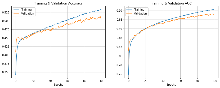
Results

Let's plot the training and validation AUC and accuracy.

fig, axs = plt.subplots(nrows=1, ncols=2, figsize=(14, 5))

axs[0].plot(range(EPOCHS), history.history["accuracy"], label="Training")
axs[0].plot(range(EPOCHS), history.history["val_accuracy"], label="Validation")
axs[0].set_xlabel("Epochs")
axs[0].set_title("Training & Validation Accuracy")
axs[0].legend()
axs[0].grid(True)

axs[1].plot(range(EPOCHS), history.history["auc"], label="Training")
axs[1].plot(range(EPOCHS), history.history["val_auc"], label="Validation")
axs[1].set_xlabel("Epochs")
axs[1].set_title("Training & Validation AUC")
axs[1].legend()
axs[1].grid(True)

plt.show()

png

Evaluation

train_loss, train_acc, train_auc = model.evaluate(train_ds)
valid_loss, valid_acc, valid_auc = model.evaluate(valid_ds)

3169/3169 [==============================] - 10s 3ms/step - loss: 1.0117 - accuracy: 0.5423 - auc: 0.9079
349/349 [==============================] - 1s 3ms/step - loss: 1.1125 - accuracy: 0.5039 - auc: 0.8907

Let's try to compare our model's performance to Yamnet's using one of Yamnet metrics (d-prime) Yamnet achieved a d-prime value of 2.318. Let's check our model's performance.

# The following function calculates the d-prime score from the AUC
def d_prime(auc):
    standard_normal = stats.norm()
    d_prime = standard_normal.ppf(auc) * np.sqrt(2.0)
    return d_prime


print(
    "train d-prime: {0:.3f}, validation d-prime: {1:.3f}".format(
        d_prime(train_auc), d_prime(valid_auc)
    )
)

train d-prime: 1.878, validation d-prime: 1.740

We can see that the model achieves the following results:

Results	Training	Validation
Accuracy	54%	51%
AUC	0.91	0.89
d-prime	1.882	1.740

Confusion Matrix

Let's now plot the confusion matrix for the validation dataset.

The confusion matrix lets us see, for every class, not only how many samples were correctly classified, but also which other classes were the samples confused with.

It allows us to calculate the precision and recall for every class.

# Create x and y tensors
x_valid = None
y_valid = None

for x, y in iter(valid_ds):
    if x_valid is None:
        x_valid = x.numpy()
        y_valid = y.numpy()
    else:
        x_valid = np.concatenate((x_valid, x.numpy()), axis=0)
        y_valid = np.concatenate((y_valid, y.numpy()), axis=0)

# Generate predictions
y_pred = model.predict(x_valid)

# Calculate confusion matrix
confusion_mtx = tf.math.confusion_matrix(
    np.argmax(y_valid, axis=1), np.argmax(y_pred, axis=1)
)

# Plot the confusion matrix
plt.figure(figsize=(10, 8))
sns.heatmap(
    confusion_mtx, xticklabels=class_names, yticklabels=class_names, annot=True, fmt="g"
)
plt.xlabel("Prediction")
plt.ylabel("Label")
plt.title("Validation Confusion Matrix")
plt.show()

png

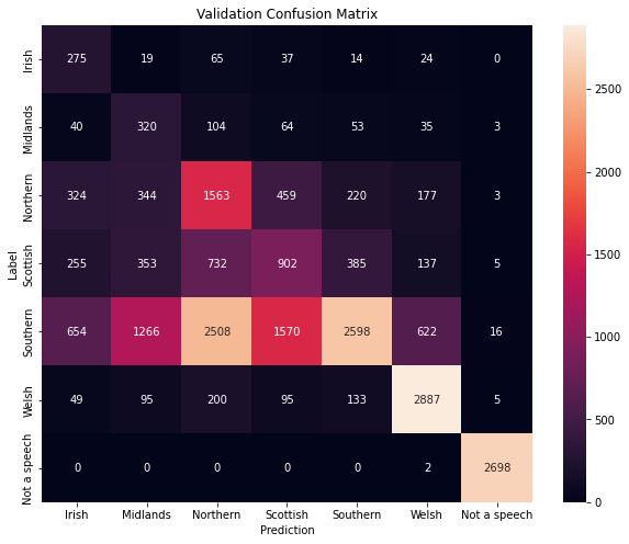
Precision & recall

For every class:

Recall is the ratio of correctly classified samples i.e. it shows how many samples of this specific class, the model is able to detect. It is the ratio of diagonal elements to the sum of all elements in the row.
Precision shows the accuracy of the classifier. It is the ratio of correctly predicted samples among the ones classified as belonging to this class. It is the ratio of diagonal elements to the sum of all elements in the column.

for i, label in enumerate(class_names):
    precision = confusion_mtx[i, i] / np.sum(confusion_mtx[:, i])
    recall = confusion_mtx[i, i] / np.sum(confusion_mtx[i, :])
    print(
        "{0:15} Precision:{1:.2f}%; Recall:{2:.2f}%".format(
            label, precision * 100, recall * 100
        )
    )

Irish           Precision:17.22%; Recall:63.36%
Midlands        Precision:13.35%; Recall:51.70%
Northern        Precision:30.22%; Recall:50.58%
Scottish        Precision:28.85%; Recall:32.57%
Southern        Precision:76.34%; Recall:28.14%
Welsh           Precision:74.33%; Recall:83.34%
Not a speech    Precision:98.83%; Recall:99.93%

Run inference on test data

Let's now run a test on a single audio file. Let's check this example from The Scottish Voice

We will:

Download the mp3 file.
Convert it to a 16k wav file.
Run the model on the wav file.
Plot the results.

filename = "audio-sample-Stuart"
url = "https://www.thescottishvoice.org.uk/files/cm/files/"

if os.path.exists(filename + ".wav") == False:
    print(f"Downloading {filename}.mp3 from {url}")
    command = f"wget {url}{filename}.mp3"
    os.system(command)

    print(f"Converting mp3 to wav and resampling to 16 kHZ")
    command = (
        f"ffmpeg -hide_banner -loglevel panic -y -i {filename}.mp3 -acodec "
        f"pcm_s16le -ac 1 -ar 16000 {filename}.wav"
    )
    os.system(command)

filename = filename + ".wav"

Downloading audio-sample-Stuart.mp3 from https://www.thescottishvoice.org.uk/files/cm/files/
Converting mp3 to wav and resampling to 16 kHZ

The below function yamnet_class_names_from_csv was copied and very slightly changed from this Yamnet Notebook.

def yamnet_class_names_from_csv(yamnet_class_map_csv_text):
    """Returns list of class names corresponding to score vector."""
    yamnet_class_map_csv = io.StringIO(yamnet_class_map_csv_text)
    yamnet_class_names = [
        name for (class_index, mid, name) in csv.reader(yamnet_class_map_csv)
    ]
    yamnet_class_names = yamnet_class_names[1:]  # Skip CSV header
    return yamnet_class_names


yamnet_class_map_path = yamnet_model.class_map_path().numpy()
yamnet_class_names = yamnet_class_names_from_csv(
    tf.io.read_file(yamnet_class_map_path).numpy().decode("utf-8")
)


def calculate_number_of_non_speech(scores):
    number_of_non_speech = tf.math.reduce_sum(
        tf.where(tf.math.argmax(scores, axis=1, output_type=tf.int32) != 0, 1, 0)
    )

    return number_of_non_speech


def filename_to_predictions(filename):
    # Load 16k audio wave
    audio_wav = load_16k_audio_wav(filename)

    # Get audio embeddings & scores.
    scores, embeddings, mel_spectrogram = yamnet_model(audio_wav)

    print(
        "Out of {} samples, {} are not speech".format(
            scores.shape[0], calculate_number_of_non_speech(scores)
        )
    )

    # Predict the output of the accent recognition model with embeddings as input
    predictions = model.predict(embeddings)

    return audio_wav, predictions, mel_spectrogram

Let's run the model on the audio file:

audio_wav, predictions, mel_spectrogram = filename_to_predictions(filename)

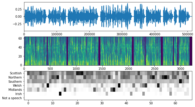
infered_class = class_names[predictions.mean(axis=0).argmax()]
print(f"The main accent is: {infered_class} English")

Out of 66 samples, 0 are not speech
The main accent is: Scottish English

Listen to the audio

Audio(audio_wav, rate=16000)

The below function was copied from this Yamnet notebook and adjusted to our need.

This function plots the following:

Audio waveform
Mel spectrogram
Predictions for every time step

plt.figure(figsize=(10, 6))

# Plot the waveform.
plt.subplot(3, 1, 1)
plt.plot(audio_wav)
plt.xlim([0, len(audio_wav)])

# Plot the log-mel spectrogram (returned by the model).
plt.subplot(3, 1, 2)
plt.imshow(
    mel_spectrogram.numpy().T, aspect="auto", interpolation="nearest", origin="lower"
)

# Plot and label the model output scores for the top-scoring classes.
mean_predictions = np.mean(predictions, axis=0)

top_class_indices = np.argsort(mean_predictions)[::-1]
plt.subplot(3, 1, 3)
plt.imshow(
    predictions[:, top_class_indices].T,
    aspect="auto",
    interpolation="nearest",
    cmap="gray_r",
)

# patch_padding = (PATCH_WINDOW_SECONDS / 2) / PATCH_HOP_SECONDS
# values from the model documentation
patch_padding = (0.025 / 2) / 0.01
plt.xlim([-patch_padding - 0.5, predictions.shape[0] + patch_padding - 0.5])
# Label the top_N classes.
yticks = range(0, len(class_names), 1)
plt.yticks(yticks, [class_names[top_class_indices[x]] for x in yticks])
_ = plt.ylim(-0.5 + np.array([len(class_names), 0]))

png

English speaker accent recognition using Transfer Learning

◆ Introduction

◆ Configuration

◆ Imports

◆ Yamnet Model

◆ Dataset

◆ Download the data

◆ Load the data in a Dataframe

◆ Prepare training & validation sets

◆ Prepare a TensorFlow Dataset

◆ Build the model

◆ Class weights calculation

◆ Callbacks

◆ Training

◆ Results

◆ Evaluation

◆ Confusion Matrix

◆ Precision & recall

◆ Run inference on test data