Automatic Speech Recognition using CTC
Authors: Mohamed Reda Bouadjenek and Ngoc Dung Huynh
Date created: 2021/09/26
Last modified: 2026/01/27
Description: Training a CTC-based model for automatic speech recognition.

Introduction
Speech recognition is an interdisciplinary subfield of computer science and computational linguistics that develops methodologies and technologies that enable the recognition and translation of spoken language into text by computers. It is also known as automatic speech recognition (ASR), computer speech recognition or speech to text (STT). It incorporates knowledge and research in the computer science, linguistics and computer engineering fields.
This demonstration shows how to combine a 2D CNN, RNN and a Connectionist Temporal Classification (CTC) loss to build an ASR. CTC is an algorithm used to train deep neural networks in speech recognition, handwriting recognition and other sequence problems. CTC is used when we don’t know how the input aligns with the output (how the characters in the transcript align to the audio). The model we create is similar to DeepSpeech2.
We will use the LJSpeech dataset from the LibriVox project. It consists of short audio clips of a single speaker reading passages from 7 non-fiction books.
We will evaluate the quality of the model using Word Error Rate (WER). WER is obtained by adding up the substitutions, insertions, and deletions that occur in a sequence of recognized words. Divide that number by the total number of words originally spoken. The result is the WER. To get the WER score you need to install the jiwer package. You can use the following command line:
pip install jiwer
References:
Setup
import pandas as pd
import numpy as np
import tensorflow as tf
import keras
from keras import layers
from keras import ops
import matplotlib.pyplot as plt
from IPython import display
from jiwer import wer
WARNING: All log messages before absl::InitializeLog() is called are written to STDERR
E0000 00:00:1770807431.103047    3901 cuda_dnn.cc:8579] Unable to register cuDNN factory: Attempting to register factory for plugin cuDNN when one has already been registered
E0000 00:00:1770807431.107368    3901 cuda_blas.cc:1407] Unable to register cuBLAS factory: Attempting to register factory for plugin cuBLAS when one has already been registered
W0000 00:00:1770807431.118439    3901 computation_placer.cc:177] computation placer already registered. Please check linkage and avoid linking the same target more than once.
W0000 00:00:1770807431.118450    3901 computation_placer.cc:177] computation placer already registered. Please check linkage and avoid linking the same target more than once.
W0000 00:00:1770807431.118451    3901 computation_placer.cc:177] computation placer already registered. Please check linkage and avoid linking the same target more than once.
W0000 00:00:1770807431.118453    3901 computation_placer.cc:177] computation placer already registered. Please check linkage and avoid linking the same target more than once.
Load the LJSpeech Dataset
Let's download the LJSpeech Dataset.
The dataset contains 13,100 audio files as wav files in the /wavs/ folder.
The label (transcript) for each audio file is a string
given in the metadata.csv file. The fields are:
- ID: this is the name of the corresponding .wav file
- Transcription: words spoken by the reader (UTF-8)
- Normalized transcription: transcription with numbers, ordinals, and monetary units expanded into full words (UTF-8).
For this demo we will use on the "Normalized transcription" field.
Each audio file is a single-channel 16-bit PCM WAV with a sample rate of 22,050 Hz.
data_url = "https://data.keithito.com/data/speech/LJSpeech-1.1.tar.bz2"
data_path = keras.utils.get_file("LJSpeech-1.1", data_url, untar=True)
wavs_path = data_path + "/LJSpeech-1.1/wavs/"
metadata_path = data_path + "/LJSpeech-1.1" + "/metadata.csv"


# Read metadata file and parse it
metadata_df = pd.read_csv(metadata_path, sep="|", header=None, quoting=3)
metadata_df.columns = ["file_name", "transcription", "normalized_transcription"]
metadata_df = metadata_df[["file_name", "normalized_transcription"]]
metadata_df = metadata_df.sample(frac=1).reset_index(drop=True)
metadata_df.head(3)
Downloading data from https://data.keithito.com/data/speech/LJSpeech-1.1.tar.bz2

2748572632/2748572632 ━━━━━━━━━━━━━━━━━━━━ 7s 0us/step
| file_name | normalized_transcription | |
|---|---|---|
| 0 | LJ049-0116 | of such persons as have been constitutionally ... |
| 1 | LJ038-0248 | was also identified by Marina Oswald as having... |
| 2 | LJ047-0129 | FBI informants in the New Orleans area, famili... |
We now split the data into training and validation set.
split = int(len(metadata_df) * 0.90)
df_train = metadata_df[:split]
df_val = metadata_df[split:]

print(f"Size of the training set: {len(df_train)}")
print(f"Size of the training set: {len(df_val)}")
Size of the training set: 11790
Size of the training set: 1310
Preprocessing
We first prepare the vocabulary to be used.
# The set of characters accepted in the transcription.
characters = [x for x in "abcdefghijklmnopqrstuvwxyz'?! "]
# Mapping characters to integers
char_to_num = keras.layers.StringLookup(vocabulary=characters, oov_token="")
# Mapping integers back to original characters
num_to_char = keras.layers.StringLookup(
    vocabulary=char_to_num.get_vocabulary(), oov_token="", invert=True
)

print(
    f"The vocabulary is: {char_to_num.get_vocabulary()} "
    f"(size ={char_to_num.vocabulary_size()})"
)
The vocabulary is: ['', np.str_('a'), np.str_('b'), np.str_('c'), np.str_('d'), np.str_('e'), np.str_('f'), np.str_('g'), np.str_('h'), np.str_('i'), np.str_('j'), np.str_('k'), np.str_('l'), np.str_('m'), np.str_('n'), np.str_('o'), np.str_('p'), np.str_('q'), np.str_('r'), np.str_('s'), np.str_('t'), np.str_('u'), np.str_('v'), np.str_('w'), np.str_('x'), np.str_('y'), np.str_('z'), np.str_("'"), np.str_('?'), np.str_('!'), np.str_(' ')] (size =31)
Next, we create the function that describes the transformation that we apply to each element of our dataset.
# An integer scalar Tensor. The window length in samples.
frame_length = 256
# An integer scalar Tensor. The number of samples to step.
frame_step = 160
# An integer scalar Tensor. The size of the FFT to apply.
# If not provided, uses the smallest power of 2 enclosing frame_length.
fft_length = 384


def encode_single_sample(wav_file, label):
    ###########################################
    ##  Process the Audio
    ##########################################
    # 1. Read wav file
    file = tf.io.read_file(wavs_path + wav_file + ".wav")
    # 2. Decode the wav file
    audio, _ = tf.audio.decode_wav(file)
    audio = ops.squeeze(audio)
    # 3. Change type to float
    audio = ops.cast(audio, "float32")
    # 4. Get the spectrogram
    stft_output = ops.stft(
        audio,
        sequence_length=frame_length,
        sequence_stride=frame_step,
        fft_length=fft_length,
        center=False,
    )
    # 5. We only need the magnitude, which can be computed from real and imaginary parts
    # stft returns (real, imag) tuple - compute magnitude as sqrt(real^2 + imag^2)
    spectrogram = ops.sqrt(ops.square(stft_output[0]) + ops.square(stft_output[1]))
    spectrogram = ops.power(spectrogram, 0.5)
    # 6. normalisation
    means = ops.mean(spectrogram, axis=1, keepdims=True)
    stddevs = ops.std(spectrogram, axis=1, keepdims=True)
    spectrogram = (spectrogram - means) / (stddevs + 1e-10)
    ###########################################
    ##  Process the label
    ##########################################
    # 7. Convert label to Lower case
    label = tf.strings.lower(label)
    # 8. Split the label
    label = tf.strings.unicode_split(label, input_encoding="UTF-8")
    # 9. Map the characters in label to numbers
    label = char_to_num(label)
    # 10. Return a dict as our model is expecting two inputs
    return spectrogram, label
Creating Dataset objects
We create a tf.data.Dataset object that yields
the transformed elements, in the same order as they
appeared in the input.
batch_size = 32
# Define the training dataset
train_dataset = tf.data.Dataset.from_tensor_slices(
    (list(df_train["file_name"]), list(df_train["normalized_transcription"]))
)
train_dataset = (
    train_dataset.map(encode_single_sample, num_parallel_calls=tf.data.AUTOTUNE)
    .padded_batch(batch_size, padded_shapes=([None, fft_length // 2 + 1], [None]))
    .prefetch(buffer_size=tf.data.AUTOTUNE)
)

# Define the validation dataset
validation_dataset = tf.data.Dataset.from_tensor_slices(
    (list(df_val["file_name"]), list(df_val["normalized_transcription"]))
)
validation_dataset = (
    validation_dataset.map(encode_single_sample, num_parallel_calls=tf.data.AUTOTUNE)
    .padded_batch(batch_size, padded_shapes=([None, fft_length // 2 + 1], [None]))
    .prefetch(buffer_size=tf.data.AUTOTUNE)
)
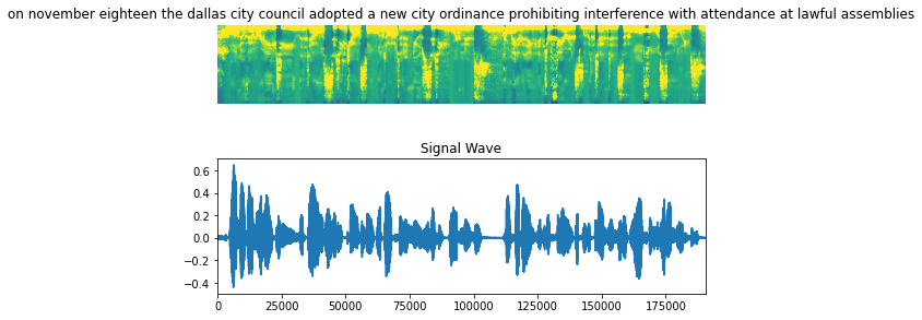
Visualize the data
Let's visualize an example in our dataset, including the audio clip, the spectrogram and the corresponding label.
fig = plt.figure(figsize=(8, 5))
for batch in train_dataset.take(1):
    spectrogram = batch[0][0].numpy()
    spectrogram = np.array([np.trim_zeros(x) for x in np.transpose(spectrogram)])
    label = batch[1][0]
    # Spectrogram
    label = tf.strings.reduce_join(num_to_char(label)).numpy().decode("utf-8")
    ax = plt.subplot(2, 1, 1)
    ax.imshow(spectrogram, vmax=1)
    ax.set_title(label)
    ax.axis("off")
    # Wav
    file = tf.io.read_file(wavs_path + list(df_train["file_name"])[0] + ".wav")
    audio, _ = tf.audio.decode_wav(file)
    audio = audio.numpy()
    ax = plt.subplot(2, 1, 2)
    plt.plot(audio)
    ax.set_title("Signal Wave")
    ax.set_xlim(0, len(audio))
    display.display(display.Audio(np.transpose(audio), rate=16000))
plt.show()
Model
We first define the CTC Loss function.
def CTCLoss(y_true, y_pred):
    # Compute the training-time loss value
    batch_len = ops.shape(y_true)[0]
    input_length = ops.shape(y_pred)[1]
    label_length = ops.shape(y_true)[1]

    # Create length tensors - CTC needs to know the actual sequence lengths
    input_length = input_length * ops.ones(shape=(batch_len,), dtype="int32")
    label_length = label_length * ops.ones(shape=(batch_len,), dtype="int32")

    # Use Keras ops CTC loss (backend-agnostic)
    # Note: mask_index should match the blank token index
    # With StringLookup(oov_token=""), index 0 is reserved, so we use 0 as mask
    loss = ops.nn.ctc_loss(
        target=ops.cast(y_true, "int32"),
        output=y_pred,
        target_length=label_length,
        output_length=input_length,
        mask_index=0,
    )
    return loss
We now define our model. We will define a model similar to DeepSpeech2.
def build_model(input_dim, output_dim, rnn_layers=5, rnn_units=128):
    """Model similar to DeepSpeech2."""
    # Model's input
    input_spectrogram = layers.Input((None, input_dim), name="input")
    # Expand the dimension to use 2D CNN.
    x = layers.Reshape((-1, input_dim, 1), name="expand_dim")(input_spectrogram)
    # Convolution layer 1
    x = layers.Conv2D(
        filters=32,
        kernel_size=[11, 41],
        strides=[2, 2],
        padding="same",
        use_bias=False,
        name="conv_1",
    )(x)
    x = layers.BatchNormalization(name="conv_1_bn")(x)
    x = layers.ReLU(name="conv_1_relu")(x)
    # Convolution layer 2
    x = layers.Conv2D(
        filters=32,
        kernel_size=[11, 21],
        strides=[1, 2],
        padding="same",
        use_bias=False,
        name="conv_2",
    )(x)
    x = layers.BatchNormalization(name="conv_2_bn")(x)
    x = layers.ReLU(name="conv_2_relu")(x)
    # Reshape the resulted volume to feed the RNNs layers
    x = layers.Reshape((-1, x.shape[-2] * x.shape[-1]))(x)
    # RNN layers
    for i in range(1, rnn_layers + 1):
        recurrent = layers.GRU(
            units=rnn_units,
            activation="tanh",
            recurrent_activation="sigmoid",
            use_bias=True,
            return_sequences=True,
            reset_after=True,
            name=f"gru_{i}",
        )
        x = layers.Bidirectional(
            recurrent, name=f"bidirectional_{i}", merge_mode="concat"
        )(x)
        if i < rnn_layers:
            x = layers.Dropout(rate=0.5)(x)
    # Dense layer
    x = layers.Dense(units=rnn_units * 2, name="dense_1")(x)
    x = layers.ReLU(name="dense_1_relu")(x)
    x = layers.Dropout(rate=0.5)(x)
    # Classification layer
    output = layers.Dense(units=output_dim + 1, activation="softmax")(x)
    # Model
    model = keras.Model(input_spectrogram, output, name="DeepSpeech_2")
    # Optimizer
    opt = keras.optimizers.Adam(learning_rate=1e-4)
    # Compile the model and return
    model.compile(optimizer=opt, loss=CTCLoss)
    return model


# Get the model
model = build_model(
    input_dim=fft_length // 2 + 1,
    output_dim=char_to_num.vocabulary_size(),
    rnn_units=512,
)
model.summary(line_length=110)
Model: "DeepSpeech_2"
┏━━━━━━━━━━━━━━━━━━━━━━━━━━━━━━━━━━━━━━━━━━━━━━━━┳━━━━━━━━━━━━━━━━━━━━━━━━━━━━━━━━━━━━━┳━━━━━━━━━━━━━━━━━━━━━┓
┃ Layer (type)                                   ┃ Output Shape                        ┃             Param # ┃
┡━━━━━━━━━━━━━━━━━━━━━━━━━━━━━━━━━━━━━━━━━━━━━━━━╇━━━━━━━━━━━━━━━━━━━━━━━━━━━━━━━━━━━━━╇━━━━━━━━━━━━━━━━━━━━━┩
│ input (InputLayer)                             │ (None, None, 193)                   │                   0 │
├────────────────────────────────────────────────┼─────────────────────────────────────┼─────────────────────┤
│ expand_dim (Reshape)                           │ (None, None, 193, 1)                │                   0 │
├────────────────────────────────────────────────┼─────────────────────────────────────┼─────────────────────┤
│ conv_1 (Conv2D)                                │ (None, None, 97, 32)                │              14,432 │
├────────────────────────────────────────────────┼─────────────────────────────────────┼─────────────────────┤
│ conv_1_bn (BatchNormalization)                 │ (None, None, 97, 32)                │                 128 │
├────────────────────────────────────────────────┼─────────────────────────────────────┼─────────────────────┤
│ conv_1_relu (ReLU)                             │ (None, None, 97, 32)                │                   0 │
├────────────────────────────────────────────────┼─────────────────────────────────────┼─────────────────────┤
│ conv_2 (Conv2D)                                │ (None, None, 49, 32)                │             236,544 │
├────────────────────────────────────────────────┼─────────────────────────────────────┼─────────────────────┤
│ conv_2_bn (BatchNormalization)                 │ (None, None, 49, 32)                │                 128 │
├────────────────────────────────────────────────┼─────────────────────────────────────┼─────────────────────┤
│ conv_2_relu (ReLU)                             │ (None, None, 49, 32)                │                   0 │
├────────────────────────────────────────────────┼─────────────────────────────────────┼─────────────────────┤
│ reshape (Reshape)                              │ (None, None, 1568)                  │                   0 │
├────────────────────────────────────────────────┼─────────────────────────────────────┼─────────────────────┤
│ bidirectional_1 (Bidirectional)                │ (None, None, 1024)                  │           6,395,904 │
├────────────────────────────────────────────────┼─────────────────────────────────────┼─────────────────────┤
│ dropout (Dropout)                              │ (None, None, 1024)                  │                   0 │
├────────────────────────────────────────────────┼─────────────────────────────────────┼─────────────────────┤
│ bidirectional_2 (Bidirectional)                │ (None, None, 1024)                  │           4,724,736 │
├────────────────────────────────────────────────┼─────────────────────────────────────┼─────────────────────┤
│ dropout_1 (Dropout)                            │ (None, None, 1024)                  │                   0 │
├────────────────────────────────────────────────┼─────────────────────────────────────┼─────────────────────┤
│ bidirectional_3 (Bidirectional)                │ (None, None, 1024)                  │           4,724,736 │
├────────────────────────────────────────────────┼─────────────────────────────────────┼─────────────────────┤
│ dropout_2 (Dropout)                            │ (None, None, 1024)                  │                   0 │
├────────────────────────────────────────────────┼─────────────────────────────────────┼─────────────────────┤
│ bidirectional_4 (Bidirectional)                │ (None, None, 1024)                  │           4,724,736 │
├────────────────────────────────────────────────┼─────────────────────────────────────┼─────────────────────┤
│ dropout_3 (Dropout)                            │ (None, None, 1024)                  │                   0 │
├────────────────────────────────────────────────┼─────────────────────────────────────┼─────────────────────┤
│ bidirectional_5 (Bidirectional)                │ (None, None, 1024)                  │           4,724,736 │
├────────────────────────────────────────────────┼─────────────────────────────────────┼─────────────────────┤
│ dense_1 (Dense)                                │ (None, None, 1024)                  │           1,049,600 │
├────────────────────────────────────────────────┼─────────────────────────────────────┼─────────────────────┤
│ dense_1_relu (ReLU)                            │ (None, None, 1024)                  │                   0 │
├────────────────────────────────────────────────┼─────────────────────────────────────┼─────────────────────┤
│ dropout_4 (Dropout)                            │ (None, None, 1024)                  │                   0 │
├────────────────────────────────────────────────┼─────────────────────────────────────┼─────────────────────┤
│ dense (Dense)                                  │ (None, None, 32)                    │              32,800 │
└────────────────────────────────────────────────┴─────────────────────────────────────┴─────────────────────┘
Total params: 26,628,480 (101.58 MB)
Trainable params: 26,628,352 (101.58 MB)
Non-trainable params: 128 (512.00 B)
Training and Evaluating
# A utility function to decode the output of the network
def decode_batch_predictions(pred):
    input_len = np.ones(pred.shape[0]) * pred.shape[1]

    # Use Keras ops CTC decoder with greedy strategy (backend-agnostic)
    decoded = ops.nn.ctc_decode(
        inputs=pred,
        sequence_lengths=ops.cast(input_len, "int32"),
        strategy="greedy",
        mask_index=0,
    )

    # ctc_decode returns a tuple of (decoded_sequences, log_probabilities)
    # For greedy strategy, decoded_sequences has shape: (1, batch_size, max_length)
    # So we need decoded[0][0] to get the batch with shape (batch_size, max_length)
    decoded_sequences = decoded[0][0]

    # Convert to numpy once for the whole batch
    decoded_sequences = ops.convert_to_numpy(decoded_sequences)

    # Iterate over the results and get back the text
    output_text = []
    for sequence in decoded_sequences:
        # Remove padding/mask values (0 is the mask index)
        sequence = sequence[sequence > 0]
        # Convert indices to characters
        text = tf.strings.reduce_join(num_to_char(sequence)).numpy().decode("utf-8")
        output_text.append(text)
    return output_text


# A callback class to output a few transcriptions during training
class CallbackEval(keras.callbacks.Callback):
    """Displays a batch of outputs after every epoch."""

    def __init__(self, dataset):
        super().__init__()
        self.dataset = dataset

    def on_epoch_end(self, epoch: int, logs=None):
        predictions = []
        targets = []
        # Limit to 10 batches to avoid long evaluation times
        for i, batch in enumerate(self.dataset):
            if i >= 10:
                break
            X, y = batch
            print(f"Batch {i}: X shape = {X.shape}, y shape = {y.shape}")
            batch_predictions = model.predict(X, verbose=0)
            print(f"Batch {i}: predictions shape = {batch_predictions.shape}")
            batch_predictions = decode_batch_predictions(batch_predictions)
            print(f"Batch {i}: decoded {len(batch_predictions)} predictions")
            predictions.extend(batch_predictions)
            for label in y:
                label = (
                    tf.strings.reduce_join(num_to_char(label)).numpy().decode("utf-8")
                )
                targets.append(label)
        print(f"\nTotal: {len(predictions)} predictions, {len(targets)} targets")
        wer_score = wer(targets, predictions)
        print("-" * 100)
        print(f"Word Error Rate: {wer_score:.4f}")
        print("-" * 100)
        for i in np.random.randint(0, len(predictions), 2):
            print(f"Target    : {targets[i]}")
            print(f"Prediction: {predictions[i]}")
            print("-" * 100)
Let's start the training process.
# Define the number of epochs.
epochs = 1
# Callback function to check transcription on the val set.
validation_callback = CallbackEval(validation_dataset)
# Train the model
history = model.fit(
    train_dataset,
    validation_data=validation_dataset,
    epochs=epochs,
    callbacks=[validation_callback],
)
369/369 ━━━━━━━━━━━━━━━━━━━━ 0s 10s/step - loss: 1379.7394

Batch 0: X shape = (32, 1370, 193), y shape = (32, 148)

Batch 0: predictions shape = (32, 685, 32)
Batch 0: decoded 32 predictions
Batch 1: X shape = (32, 1373, 193), y shape = (32, 159)

Batch 1: predictions shape = (32, 687, 32)
Batch 1: decoded 32 predictions
Batch 2: X shape = (32, 1389, 193), y shape = (32, 167)

Batch 2: predictions shape = (32, 695, 32)
Batch 2: decoded 32 predictions
Batch 3: X shape = (32, 1327, 193), y shape = (32, 162)

Batch 3: predictions shape = (32, 664, 32)
Batch 3: decoded 32 predictions
Batch 4: X shape = (32, 1373, 193), y shape = (32, 165)

Batch 4: predictions shape = (32, 687, 32)
Batch 4: decoded 32 predictions
Batch 5: X shape = (32, 1354, 193), y shape = (32, 149)

Batch 5: predictions shape = (32, 677, 32)
Batch 5: decoded 32 predictions
Batch 6: X shape = (32, 1388, 193), y shape = (32, 168)

Batch 6: predictions shape = (32, 694, 32)
Batch 6: decoded 32 predictions
Batch 7: X shape = (32, 1381, 193), y shape = (32, 171)

Batch 7: predictions shape = (32, 691, 32)
Batch 7: decoded 32 predictions
Batch 8: X shape = (32, 1383, 193), y shape = (32, 155)

Batch 8: predictions shape = (32, 692, 32)
Batch 8: decoded 32 predictions
Batch 9: X shape = (32, 1386, 193), y shape = (32, 149)

Batch 9: predictions shape = (32, 693, 32)
Batch 9: decoded 32 predictions

Total: 320 predictions, 320 targets
----------------------------------------------------------------------------------------------------
Word Error Rate: 1.0000
----------------------------------------------------------------------------------------------------
Target    : they set out but at leeds wakefield found himself called suddenly to paris
Prediction:
----------------------------------------------------------------------------------------------------
Target    : would have seemed somewhat serious to us even though i must admit that none of these in themselves would be
Prediction:
----------------------------------------------------------------------------------------------------
369/369 ━━━━━━━━━━━━━━━━━━━━ 4065s 11s/step - loss: 1362.6790 - val_loss: 1365.2762
Inference
# Let's check results on more validation samples
predictions = []
targets = []
for batch in validation_dataset:
    X, y = batch
    batch_predictions = model.predict(X)
    batch_predictions = decode_batch_predictions(batch_predictions)
    predictions.extend(batch_predictions)
    for label in y:
        label = tf.strings.reduce_join(num_to_char(label)).numpy().decode("utf-8")
        targets.append(label)
wer_score = wer(targets, predictions)
print("-" * 100)
print(f"Word Error Rate: {wer_score:.4f}")
print("-" * 100)
for i in np.random.randint(0, len(predictions), 5):
    print(f"Target    : {targets[i]}")
    print(f"Prediction: {predictions[i]}")
    print("-" * 100)
1/1 ━━━━━━━━━━━━━━━━━━━━ 4s 4s/step

----------------------------------------------------------------------------------------------------
Word Error Rate: 1.0000
----------------------------------------------------------------------------------------------------
Target    : parts of the walls of nineveh are still standing to the height of one hundred and twentyfive feet
Prediction:
----------------------------------------------------------------------------------------------------
Target    : on the return flight mrs kennedy sat with david powers kenneth o'donnell and lawrence o'brien
Prediction:
----------------------------------------------------------------------------------------------------
Target    : so that i know not where we can hope to find any absolute distinction between animals and plants unless we return to their mode of nutrition
Prediction:
----------------------------------------------------------------------------------------------------
Target    : testified that she was quote quite hysterical end quote and was quote crying and upset end quote
Prediction:
----------------------------------------------------------------------------------------------------
Target    : and was investigating him at the time of the assassination the commission has taken the testimony of bureau agents
Prediction:
----------------------------------------------------------------------------------------------------
Conclusion
In practice, you should train for around 50 epochs or more. Each epoch
takes approximately 8-10 minutes using a Colab A100 GPU.
The model we trained at 50 epochs has a Word Error Rate (WER) ≈ 16% to 17%.
Some of the transcriptions around epoch 50:
Audio file: LJ017-0009.wav
- Target    : sir thomas overbury was undoubtedly poisoned by lord rochester in the reign
of james the first
- Prediction: cer thomas overbery was undoubtedly poisoned by lordrochester in the reign
of james the first
Audio file: LJ003-0340.wav
- Target    : the committee does not seem to have yet understood that newgate could be
only and properly replaced
- Prediction: the committee does not seem to have yet understood that newgate could be
only and proberly replace
Audio file: LJ011-0136.wav
- Target    : still no sentence of death was carried out for the offense and in eighteen
thirtytwo
- Prediction: still no sentence of death was carried out for the offense and in eighteen
thirtytwo
Example available on HuggingFace.
| Trained Model | Demo |
| :–: | :–: |
| ![]()